J. Cent. South Univ. Technol. (2008) 15: 256-263
DOI: 10.1007/s11771-008-0048-1

Compensation for secondary uncertainty in electro-hydraulic servo system by gain adaptive sliding mode variable structure control
ZHANG You-wang(张友旺)1, GUI Wei-hua(桂卫华)2
(1. School of Mechanical and Electrical Engineering, Central South University, Changsha 410083, China;
2. School of Information Science and Engineering, Central South University, Changsha 410083, China)
Abstract: Based on consideration of the differential relations between the immeasurable variables and measurable variables in electro-hydraulic servo system, adaptive dynamic recurrent fuzzy neural networks(ADRFNNs) were employed to identify the primary uncertainty and the mathematic model of the system was turned into an equivalent linear model with terms of secondary uncertainty. At the same time, gain adaptive sliding mode variable structure control(GASMVSC) was employed to synthesize the control effort. The results show that the unrealization problem caused by some system’s immeasurable state variables in traditional fuzzy neural networks(TFNN) taking all state variables as its inputs is overcome. On the other hand, the identification by the ADRFNNs online with high accuracy and the adaptive function of the correction term’s gain in the GASMVSC make the system possess strong robustness and improved steady accuracy, and the chattering phenomenon of the control effort is also suppressed effectively.
Key words: electro-hydraulic servo system; adaptive dynamic recurrent fuzzy neural network(ADRFNN); gain adaptive sliding mode variable structure control(GASMVSC); secondary uncertainty
1 Introduction
Utilizing the adaptive fuzzy neural networks that combine the learning function of neural networks and fuzzy system’s integration function of expert experience knowledge to identify the primary uncertainty is an ideal method, and the primary uncertainty is the unknown dynamic characteristics including structure and parameter uncertainty, unmodeled dynamics, nonlinearity and load disturbance caused by variations of working point and environment in electro-hydraulic servo system. The stability and robustness of the whole system can hardly be guaranteed, if the weights and parameters of the networks are adjusted by the traditional BP methods. So the methods based on Lyapunov stability theory were extensively adopted[1-6]. And the identification errors, being called secondary uncertainty here, exist. Sliding mode variable structure control (SMVSC) or adding an additional variable structure control(VSC) term can suppress the secondary uncertainty, but its bound used to determine the correction term’s gain of the SMVSC or VSC must be known[7-11]. In practice, the correction term’s gain is selected conservatively to guarantee the robustness of system. This may make the chattering of system become serious. So the method of estimating the gain online was proposed[12], but all the state variables of the system must be measurable, and it is hard to be realized. High gain state estimator based on variable structure was proposed[13], but its estimation errors may be transferred into the neural networks and make the identification errors become larger. In fact, the degree of the chattering caused by SMVSC is related closely to the correction term’s gain of the SMVSC determined according to the bound of the secondary uncertainty, so it is necessary to adopt high accurate and realizable identification tool for the primary uncertainties to obtain smaller secondary uncertainties, and evaluate the bound of the secondary uncertainties online to determine accordingly the gain of the VSC. In this work, based on the knowledge above, the adaptive dynamic recurrent fuzzy neural network (ADRFNN), in which only measurable variables are taken as its inputs and the dynamic relations between the immeasurable variables and measurable variables are represented by its inner feedback matrix, was utilized to identify the primary uncertainty with high accuracy,so the secondary uncertainty becomes smaller and the realization of system also become easy. At the same time, gain adaptive sliding mode variable structure control (GASMVSC) was employed to estimate the bound of the secondary uncertainty online, and the correction term’s
gain was determined accordingly.
2 ADRFNN and its model
It is well known that many systems can be described by affine nonlinear system whose states have differential relations between each other, if the states are selected suitably. So the states can be described by each other through differentiating operator, especially in control engineering, the immeasurable states can be described by measurable states through differentiating operator. Based on this knowledge, ADRFNN shown in Fig.1 is proposed. It has dynamic recurrent characteristics and describes the system’s inner dynamic relations between the states by its feedback relations between the inner neurons, and takes only some measurable variables as its inputs. So it is suitable for identifying such affine nonlinear system as above.
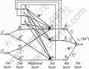
Fig.1 Schematic illustration of ADRFNN
The neurons in the first layer are connected directly with the input vector xN and transfer them to the next layer.
The neurons in the second layer represent the linguistic variables and calculate the membership values of the input variables to the linguistic variables’ fuzzy sets:
 (1)
(1)
where  is the eigenvalue of the ith input variable to the jth linguistic variable, i=1, 2, ???, nN, nN is the dimension of the input vector xN, j=1, 2, ???, mi, mi is the number of the fuzzy sets of
 and sij stand for the center and the width of the membership functions.
Every neuron in the third layer represents one fuzzy rule, mates the antecedent parts of the fuzzy rules and calculates the fired values of every rule:
 (2)
(2)
ac,j(k)=aj(k-1) (3)
 (4)
(4)
The above equations show that the fired values in the kth instant include not only the fired values  calculated from the kth instant input vector xN, but also the fired value’s contribution in the (k-1)th instant. The units in this layer adopt sigmoid activation function as shown in Eqn.(4).
The forth layer carries out the unitary calculation, that is
 l=1, 2, ???, m (5)
The fifth layer is the output layer, and it carries out the function of defuzzification calculation.
 (6)
(6)
where  is the center value of the lth membership function of the output variable.
Fig.1 shows that a unique structural unit is used to memorize the fired values of the last instant in ADRFNN, it is equivalent to a tapped delay operator.
3 GASMC based on identification by ADRFNN
3.1 Experiment system
The experiment system used to verify the effectiveness of the proposed control algorithm is shown in Fig.2, and its main component parts are as follows.
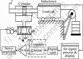
Fig.2 Schematic diagram of experiment system
3.1.1 Servo valve and its amplifier
QDY-10 servo valve and its mated amplifier were used in the experiment system. Its flow is 125 L/min if the source pressure is 6.3 MPa and no load is added. If the control voltage ranges from -10 to +10 V, the current in the range from -80 to +80 mA is transferred from the servo amplifier to the torque motor of the servo valve.
3.1.2 Cylinder
The diameter of the piston of the cylinder is 63 mm, the diameter of the piston rod is 40 mm, and the effective stroke is 305 mm.
3.1.3 Displacement detector
The displacement detector is composed of a GZZ-1 inductosyn and a SF-13 instrument for magnet stimulation and digital display, its measurement stroke is 350 mm, and its resolution is 2 mm.
3.1.4 Data acquisition card
AC1056 data acquisition card was used in this experiment system.
3.1.5 Microprocessor, operating system and program language
The CPU of the computer is Celeron 1.7 GHz, the operating system is Windows 2000, the control program edited by Matlab6.3 was turned into VC++6.0 source program by tool software Matcom to satisfy the real time need of the system.
3.2 Mathematic model of experiment system
The mathematic model of the electro-hydraulic system is mainly composed of the following three equations.
3.2.1 Flow equation of servo valve
The flow equation of servo valve is described as
 (7)
(7)
 (8)
(8)
where Cd is the discharge coefficient, w is the area gradient, ps is the oil source’s pressure, pL is the load pressure, r is the fluid mass density, xv is the displacement of the spool in the servo valve, and it is proportional to the control effort u to the amplifier of the servo valve, that is xv=Kxu, g′(pL) is defined as the flow gain of the servo valve. Eqn.(7) shows the gain g′(pL) between the load flow QL and the control effort u is the nonlinear function of load pressure pL, and it is related to the working condition, the structure of the valve, and the accuracy of manufacturing and assemblage that is hardly determined in practice, so the flow gain function g′(pL) is nonlinear and uncertain.
3.2.2 Continuity equation of cylinder
The continuity equation of the cylinder is
 (9)
(9)
where Ctc is the total leakage coefficient of cylinder, A is the effective area of piston, y is the displacement of the load car, Vt is the total compressed volume and be is the effective bulk modulus of the system, which is affected by the percentage of the air to the fluid and the pressure, and the relation is nonlinear.
3.2.3 Force balance equation of cylinder
The force balance equation of the cylinder is
 (10)
(10)
where m is the total mass of the piston and the load, Bc is the viscous friction coefficient of the piston and load, KL is the load spring constant and FL is the load force.
The complexity of pipeline makes it difficult to determine the inertia force of fluid, and the viscous friction coefficient Bc is related to the temperature of the oil, the motion status of system and the fit status of the kinematical pair. These factors are uncertain.
Taking  as the state variables, the state space description for the experiment system can be obtained from Eqns.(7, 9-10).

 (11)
(11)
where


f(x) is represented as f0(x) if all para-
meters in it are nominal values. If the variation of f(x) caused by the variations of the parameters and other uncertainties is defined as fD(x), f(x) can be represented as f(x)=f0(x)+ fD(x).
Define  , Eqn.(10) shows
that load pressure pL is the function of state vector x when the load force is zero. So g(pL) can be interpreted as g(x). g(x) is g0(x) if the load pressure pL is at the rated working point. The variation of g(x) caused by the departure of the load pressure pL from the rated working point and other uncertainties is defined as gD(x), g(x) can be described as g(x)=g0(x)+gD(x).
Assuming ,then system
(11) becomes
 (12)
(12)
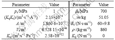
The nominal values of the parameters of the experiment system shown in Fig.1 are listed in Table 1.
Table 1 Nominal values of experiment system’s parameters
3.3 Design of GASMC
By extending system (12) to n-order affine nonlinear system, defining yd as the desired trajectory and E= 
 where yd is the desired displacement, the following error dynamic can be obtained:
 (13)
(13)
where 
 k=[kn, kn-1, ???, k1]T, k is selected to guarantee sn+k1sn-1+???+ kn to be Hurwitz polynomial.
The functions fD(x) and gD(x) are functions of the state vector x whose elements have differential relations between each other, so only the variable x1 is taken as the input of ADRFNN to estimate them. Assuming 
 and
and  are the optimal approximations for functions fD(x) and gD(x) respectively,
  and
and  are the corresponding optimal parameters of ADRFNN. Defining parameter vectors
  and
and  are the estimation values of and
  respectively, and the least approximation errors are defined as
 and
and 
Expressing  and
and  by Taylor series expansion around and yields
(14)

where
 and
and and
and 
is higher order term. By arranging Eqn.(14), the following equation can be obtained:
 (15)
(15)
Similarly, the following equation can be obtained:
 (16)
(16)
Substituting Eqns.(15-16) into Eqn.(13) and considering
 (17)
(17)
The error dynamic system (13) can be turned into
 (18)
(18)
Matrices L and B are known, and the corresponding variables in Eqn.(17) are also known through the identification by ADRFNN, so the nominal system of the error dynamic system (18) can be viewed as
 (19)
(19)
Known from the selection rule for k, L is a stable matrix. There exists a positive-definite symmetric matrix Q that makes the following Lyapunov equation
LTP+PL= -Q (20)
have a unique solution P, so a switching plane can be defined as[14]
s =SE (21)
where S=BTP, and by solving the equation
 SLE+SBueq=0 (22)
The equivalent control effort ueq of the nominal system (19) can be obtained as
ueq=-(SB)-1SLE (23)
If u′=ueq holds, the following equation can be obtained from Eqn.(17)
 (24)
(24)
 (25)
(25)
 (26)
(26)
If u′?ueq holds, and assume  then Eqns.(25-26) become
 (27)
(27)
 (28)
(28)
If the terms  in Eqn.(27) and
  in Eqn.(28) are viewed as disturbance,
and combined into the disturbance d in Eqn.(26), the following equation yields
 (29)
(29)
And Eqns.(27-28) become
 (30)
(30)
 (31)
(31)
Then Eqn.(18) turns into
 (32)
(32)
Assume:
1) dt≤d0
2)  ≤wf,
≤wf,  +
+ +d0≤
+d0≤
3)  ≤wg,
≤wg,  +
+ ≤eg
≤eg
hold,then the following inequality holds
|h2|≤efd+eguc= j (33)
where
 [efd eg]T and j=[1 |uc|].
If disturbances h1 and h2 exist in system, the control effort u′ can be selected as the following equation to strengthen the robustness of the system.
 φsign(σ)=-(SB)-1SΛE-
 φsign(σ) (34)
φ
E
where  is the estimation value of
  defining
 and assuming
  hold.
hold.
φ
E
The corresponding practical control effort u can be obtained from Eqn.(17)
 (35)
(35)
3.4 Adaptive laws and stability analysis
φ
Theorem 1 For the error dynamic system (13), if the control effort u is decided by Eqn.(35), and the adaptive laws for ADRFNN’s adjustable parameter vector and the correction term’s gain of the SMC are selected as
 (36)
(36)
 (37)
(37)
 (38)
(38)
Then the error dynamic system (13) is asymptotically stable, where
 and
and are positive adaptive gain matrices.
Proof: The following candidate Lyapunov function is considered
 (39)
(39)
And by differentiating it with respect to time, considering Eqns.(21) and (32), and taking some arrangement steps, the following equation yields:
 (40)
(40)
By substituting Eqns.(30-31) and adaptive laws Eqns.(36-37) into Eqn.(40) and considering the situation that s is a scalar, the following equation can be obtained:

φ
φ
φ
φ
φ
The following inequality can be obtained from inequality (33).
 ≤
≤ ≤
≤
 (41)
(41)
 ≤0 can be obtained by substituting adaptive law Eqn.(38) into the above inequality. By Lyapunov stability
theory,  holds. Since the switching plane is stable,
  is satisfied, and the error dynamic
system (13) is asymptotically stable. This completes the proof.
The GASMVSC algorithm based on the identification by ADRFNN is shown in Fig.3.
3.5 Analysis on experiment results
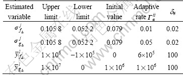
Some relevant variables for estimating the parameters s# and  of ADRFNN are listed in Table 2. Other parameters are m1=5, μ=12, k=[200, 50, 6]T, Q= diag(100, 100, 100). The displacement detector used in experiment system is incremental inductosyn, so a limit end of the cylinder is selected as the measurement original to position the system easily. But the original for modeling the valve controlled system is the middle of the cylinder, the input variable x1 of ADRFNN should be obtained by subtracting 0.15 m from the practical displacement of the load car, and the desired trajectory yd(t) is dealt with in the same way. Then the centre values of membership function are selected as
  [-0.2, -0.1, 0, 0.1, 0.2]; g0(x)=1.147 6×10⁶, f0(x)=[0, -1.42×10⁵, -16.92]x; the parameters related to the gain of SMVSC
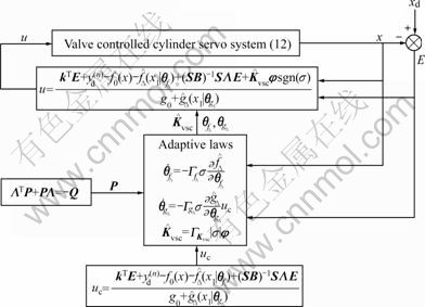
Fig.3 Frame diagram of GASMVSC based on identification by ADRFNN
Table 2 Some relevant variables for estimating parameters s# and of ADRFNN (i=j=l=1, 2, ???, m1, # stands for fD or gD)
are and its definition is given in Ref.[15]; Kvsc(0)=[1.6×10⁴, 104]T,
  diag(6×10⁴, 6×10⁴). Fig.1 shows that ADRFNN becomes traditional fuzzy neural network(TFNN) if the weights in the structural layer are set to be zero, then the initial values of all the elements of
  and
and  are set to be zero. Mwf=10, Mwg = 5,
  20,
20,  10, and their definitions are also in Ref.[15], x(0)=[0, 0, 0]T. The desired trajectory is yd(t)=0.15+0.1sin(0.1πt). The experiment results of the GASMVSC based on the identification by ADRFNN under the condition of different oil source pressures and load forces are shown in Fig.4. To compare the effect of the identification accuracy of ADRFNN and TFNN on the chattering of control effort, the experiment result by GASMVSC based on the identification by TFNN is shown in Fig.5 and that by constant gain SMVSC based on the identification by ADRFNN is shown in Fig.6.
3.5.1 Robustness of system
Figs.4-6 show that the cylinder has sine motion with 0.15 m as its center, but the control effort u is asymmetrical to the 0 V line, which results from the compensation of GASMVSC based on the identification by ADRFNN for the valve spool’s error caused during manufacturing and assemblage processes. Figs.4(a) and
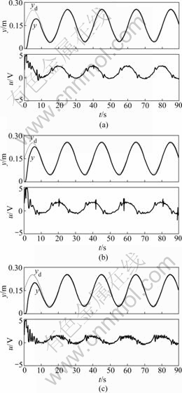
Fig.4 Experiment results by GASMVSC based on identifica- tion by ADRFNN: (a) ps=1 MPa, FL=0; (b) ps=1 MPa, FL= 500 N; (c) ps=2 MPa, FL=0
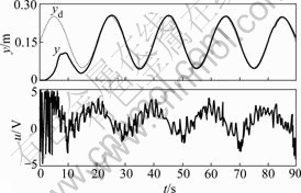
Fig.5 Experiment results by GASMVSC based on identifica- tion by TFNN (ps=1 MPa, FL=0)
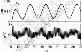
Fig.6 Experiment results by constant gain SMVSC based on identification by ADRFNN (ps=1 MPa, FL=0)
(b) show that the load force FL has no effect on tracking accuracy of system, but the curves of the control effort move up wholly, which results from the fact that stronger control efforts are needed in the drag stroke and weaker control effort is needed in the pull stroke. Figs.4(b) and (c) show that the amplitude of the control effort becomes smaller when the pressure of the oil source increases, the reason is that the gain of the system increases with the increase of oil source pressure and smaller control effort u can obtain the corresponding flow. Even so, the tracking accuracy of system is unaffected. These cases fully verify the proposed GASMVSC can make the system possess strong robustness.
3.5.2 Chattering of control effort
Figs.4 and 5 show that if the same control algorithm is used, the one based on the identification by ADRFNN has smaller amplitude of chattering of control effort than that based on the identification by TFNN, the reason is that the system identified by ADRFNN has smaller secondary uncertainty, so the correction control gain of SMVSC determined by it is smaller, which makes the amplitude of the chattering smaller. Figs.4 and 6 show that if the correction gain of SMVSC is constant, the amplitude of the chattering will hold constant. If GASMVSC is adopted, the amplitude of the chattering will become very small after adjustment for some time in the starting phase. This fact verifies the proposed GASMVSC can auto-adjust the correction gain of SMVSC according to the bound of the secondary uncertainty of system and suppress the chattering of the control effort.
3.5.3 Steady error of system
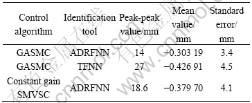
The steady displacement errors of load car (30 min later from the start point) identified and controlled by different methods are shown in Fig.7, and their statistic parameters are listed in Table 3. Fig.7 and Table 3 show that the steady accuracy of the system identified by ADRFNN is better than that identified by TFNN, and if ADRFNN is adopt as the same identification tool, the steady accuracy of system controlled by GASMVSC is better than that by constant gain SMVSC.
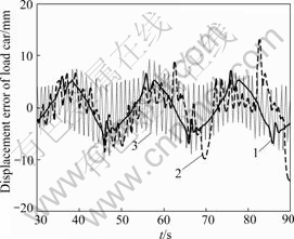
Fig.7 Steady displacement error of load car: 1―Identification by DRFNN and controlled by GASMVSC; 2―Identification by TFNN and controlled by GASMVSC; 3―Identification by DRFNN and controlled by constant gain SMVSC
Table 3 Statistic parameters of steady displacement error of load car
4 Conclusions
1) Based on the identification by ADRFNN, GASMVSC can compensate for the system parameter uncertainty and load disturbance, make the electro- hydraulic displacement tracking system possess strong robustness and good tracking performance.
2) GASMVSC can adjust its control gain automatically according to the estimated value of the bound of the second uncertainty, so smaller control effort can obtain the same robustness.
3) Identification tool with high accuracy is helpful to suppress the chattering phenomena.
References
[1] HUANG S N, TAN K K, LEE T H. Further results on adaptive control for a class of nonlinear systems suing neural networks[J]. IEEE Transactions on Neural Networks, 2003, 14(3): 719-722.
[2] LI Y, QIANG S, ZHUNG X, KAYNAK O. Robust and adaptive backstepping control for nonlinear systems using rbf neural networks[J]. IEEE Transactions on Neural Networks, 2004, 15(3): 693-701.
[3] CALISE A J, HOVAKIMYAN N, IDAN M. Adaptive output feedback control of nonlinear systems using neural networks[J]. Automatica, 2001, 37(8): 1201-1211.
[4] HOVAKIMYAN N, NARDI F, CALISE A J, KIM N. Adaptive output feedback control of uncertain nonlinear systems using single-hidden-layer neural networks[J]. IEEE Transactions on Neural Networks, 2002, 13(6): 1420-1431.
[5] GE S S, ZHANG J. Neural-network control of nonaffine nonlinear system with zero dynamics by state and output feedback[J]. IEEE Transactions on Neural Networks, 2003, 14(4): 900-918.
[6] POLYCARPOU M U, MEARS M J. Stable adaptive tracking of uncertain systems using nonlinearly parameterized on-line approximators[J]. International Journal of Control, 1998, 70(3): 363-384.
[7] BONCHIS A, CORKE P I, RYE D C, HA Q P. Variable structure methods in hydraulic servo systems control[J]. Automatica, 2001, 37(4): 589-595.
[8] TSAI C H, CHUNG H Y, YU F M. Neural-sliding mode control with its application to seesaw systems[J]. IEEE Transactions on Neural Networks, 2004, 15(1): 124-134.
[9] PARK J H, PARK G T. Robust adaptive fuzzy controller for nonlinear system using estimation of bounds for approximation errors[J]. Fuzzy Sets and System, 2003, 133(1): 19-36.
[10] FUNG R F, YANG R T. Application of VSC in position control of a nonlinear electrohydraulic servo system[J]. Computers and Structures, 1998, 66(4): 365-372.
[11] CAI Zi-xing, DUAN Zhuo-hua, ZHANG Hui-tuan, YU Jin-xia. Identification of abnormal movement state and avoiclance strategy for mobile robots [J]. J Cent South Univ Technol, 2006, 13(6): 683-688.
[12] PARK J H, HUH S H, KIM S H, SEO S J, PARK G T. Direct adaptive controller for nonaffine nonlinear systems using self-struture neural networks[J]. IEEE Transactions on Neural Networks, 2005, 16(2): 414-422.
[13] ELSHAFEI A L, KARRAY F. Varible-structue-based fuzzy-logic identification of a class of nonlinear system[J]. IEEE Transaction on Control Systems Technology, 2005, 13(4): 646-653.
[14] TIAN Hong-qi. Sliding mode control theory and its application[M]. Wuhan: Wuhan Press, 1995. (in Chinese)
[15] ZHANG You-wang, GUI Wei-hua, ZHAO Quan-ming. Adaptive electro-hydraulic position tracking system based on dynamic recurrent fuzzy neural network[J]. Control Theory and Applications, 2005, 22(4): 551-556. (in Chinese)
(Edited by CHEN Wei-ping)
Foundation item: Project(60634020) supported by the National Natural Science Foundation of China
Received date: 2007-05-11; Accepted date: 2007-06-29
Corresponding author: ZHANG You-wang, PhD; Tel: +86-13017388451; E-mail: ywzhang@mail.csu.edu.cn

