J. Cent. South Univ. (2016) 23: 150-159

DOI: 10.1007/s11771-016-3058-4

A method for improving graph queries processing using positional inverted index (P.I.I) idea in search engines and parallelization techniques

Hamed Dinari, Hassan Naderi

Web and Search Engines Laboratory, School of Computer Engineering,

Iran University of Science and Technology, Tehran, Iran

Central South University Press and Springer-Verlag Berlin Heidelberg 2016

Abstract: The idea of positional inverted index is exploited for indexing of graph database. The main idea is the use of hashing tables in order to prune a considerable portion of graph database that cannot contain the answer set. These tables are implemented using column-based techniques and are used to store graphs of database, frequent sub-graphs and the neighborhood of nodes. In order to exact checking of remaining graphs, the vertex invariant is used for isomorphism test which can be parallel implemented. The results of evaluation indicate that proposed method outperforms existing methods.

Key words: graph query processing; frequent subgraph; graph mining; data mining; positional inverted index

1 Introduction

Graphs are highly useful in different fields to display objects and the relationship between them. In science, for instance, graphs are used to model molecular structures of chemical components, food chain, and social networks [1–5]. In addition, graphs are used to show telecommunication connections, utility grids, road systems between cities, abnormalities of network [6], and indexing graphs for graph query processing [1, 7–10]. When it comes to computer graph, several usages for graphs come to mind including E-R diagram design of database, automata theory, graphical modeling in artificial intelligence (AI), and UML diagrams in software engineering. In addition, graphs can be used to model accelerating expansion of websites [11] and XML documents [12–13]. Clearly, then, graph database will find wider usages in the future. Efficient graph query processing on graph database is one of the main areas of graph mining, which is widely used in different fields. Graph mining refers to extracting useful patterns and information out of graphs [14–17]. It can be helpful for faster graph query processing. Additionally, graph indexing is used for graph query processing [1, 7–10]. Assume D={g₁, g₂, …, g_N} as a graph database including N graphs, then a graph query processing is defined: a graph query q is given, all  where g_i is a subgraph of q, are returned as a member of answer set. In general, graph query processing is featured with complex computation as all the subgraphs of a graph in the database are tested for isomorphism. Given the large number of subgraphs found in database graphs, and that isomorphism test of graph is time consuming process, graph processing is classified as NP-complete problem [18]. In general, graph query processing is complicated and time consuming. In addition, it is notable that in practice several queries are submitted to a graph database, which considerably increases complicacy of the process. Therefore, graph query processing through reading the whole database D to check if q is a subgraph of g_i is unfeasible. To solve this problem, the graph databases (such as relational database) are indexed. Several techniques for graph query processing have been proposed in the recent years. In general, query processing is carried out through two stages:

(1) Filtering: the generated index is used to filter part of the database and a set of candidate answers is generated.

(2) Candidate verification: each element of the candidate set is checked regarding presence of queried graph.

Still, complicated isomorphism tests and large candidate sets in some cases boost the costs of database query. For instance, in some cases, the set of candidate answers is almost equal with the set of definite answer set. Consequently, number of isomorphism tests increases when the answer set is large. Graph database is a new field and several studies are carried out to improve graph query performance.

In the present work, a method is proposed to facilitate graph query processing. The main idea behind the proposed method is to generate a candidate answer set as close as possible to the final answer set. Consequently, number of isomorphism tests is minimized. To this end, and to improve query pace, information retrieving techniques, i.e. inverted index, were used. The proposed method utilizes positional inverted index (P.I.I). In addition, the proposed method is featured with a specific data structure that stores graphs, nodes, communication and information needed for the query. The data structure is implemented using column-based technique (i.e. when key/value technique is not effective in a hash table, the value section of the table is implemented as key/value). In addition, graph query processing is done based on detecting frequent subgraphs and assigning more weight to them. Frequent subgraph refers to the graphs that are observed more than or equal with a threshold number (operator defined). The proposed method is a two-stage method so that the final answer might be achieved in stages depending on characteristics of the query and graphs.

The pace of query processing exceeds that of FG-index, one of fastest methods by generating inverted index and the clues needed in the data structure (see the evaluation and results). Two advantages of the proposed method including small volume of generated index and parallelism (using threads for implementation) provide outstanding information retrieving speed. Moreover, the proposed method uses vertex invariant method, a fast method for isomorphism method for isomorphism test [19]. Some of the terms and expression are defined for those readers not familiar with the concept of graph query processing.

Definition 1: A graph is displayed as G(V, E), where V stands for a set of vertex and  is a set of edges that connect the vertex.

Definition 2: Subgraph: suppose two graphs G₁(V₁, E₁, L_v1, L_E1, φ_v1, φ_E1) and G₂(V₂, E₂, L_v2, L_E2, φ_v2, φ_E2), where G₁ and G₂ are the subgraphs that meet the following conditions:

(1)

(2)

In addition, G₂ is a supergraph of G₁.

Definition 3: Isomorph graph: two graphs are isomorph when there is one-by-one correspondence between the vertex and the edges. For instance, graphs G and H are isomorphs when the following conditions are met:

With for all x, y in V→V′Φ

Definition 4: Single graph database: the data are represented as a super-graph (e.g. Facebook, Twitter, Google+, or telecommunication connections).

Definition 5: Transaction graph database: The data are represented as a set of several independent graphs (e.g. protein, amino acids, and chemical/biological informatics databases).

Definition 6: Support: the number of possible repetition modes of pattern S in graph database G. For instance, suppose freq(S) stands for number of possible repetitions of pattern S in the database, and |D| stands for the database size, then Sup is defined as

                        (1)

In this type of support, freq(s) is equal with number of graphs where the pattern S takes place. In addition, pattern S is counted once even when it appears in a graph for several times.

2 Related works

Several methods have been proposed for graph query processing. In 1976, a graph query processing technique was proposed in which the whole graph would be scanned and then the query would be tested with all subgraphs for isomorphism [20]. This method is too slow and far away from optimum storage usage. In addition, it fails to process query in large databases. WILLIAMS (2007) proposed GD index, in which the subgraphs of the graph database are extracted first and then converted to a unique string using standard codes extracted from an adjacency matrix. However, large number of subgraphs imposes great time and storage demand [21]. Afterward, GIUGNO and SHASHA [22] introduced GraphGrep technique, which was a path-based method. The technique uses path indexing to filter part of the database that the query answer cannot be there. A disadvantage of this technique is that it needs large storage space to store the paths. In light of these problems, Cindex was introduced [23], in which the frequent sub-trees are examined and indexed based on an operator-defined threshold. An advantage of this method is its better performance of pruning compared with path-based method; however, the query space might need candidate recheck during pruning process. YAN et al [10] introduced Gindex technique, in which frequent subgraphs are mined to a specific threshold and then stored in a hashed table based on standard codes. An advantage of this method is that it generates query answer faster when the query is part of frequent subgraphs; otherwise, the query occurs in few graphs in the database. In this way, a large space is pruned; number of isomorphism tests is decreased, and query pace is accelerated. FG-index was proposed, where frequent subgraphs are mined within the threshold defined by operation and stored in an inverted index [24-25]. However, when the frequent query is not maximized, the isomorphism test must be performed on the input query. An advantage of this method is reduction of index volume to a specific level [1].

3 Proposed method

The proposed method is classified in mining based graph query processing, featured with two main stages: (1) index construction, and (2) query processing.

The index is used to prune part of the query space that the query answer cannot be there. The index is generated by pre-processing on the database, and then, a set of features and patters are extracted. The extracted features and patterns are stored based on P.I.I of search engine, which has the advantage that the added graphs to the database do not need to be regenerated and merely an index update is carried out. To accelerate attaining the elements of P.I.I, hash tables and column-based technique are used (i.e. when key/value technique is not effective in a hash table, the value section of the table is implemented as key/value) to generate the tables. The structures of the data used from generating the index are as follows:

(1) Inverse list, where all bridges are arranged based on lexicographic order and stored in the graphs along with graph No. and the place of occurrence.

(2) Neighbors list where each node is stored along with its neighbors.

(3) A table is used to store the frequent subgraphs. The subgraphs are mined using gSpan algorithm [26]. At first, all the input graphs are converted to a unique string based on the smallest lexicographic sequence and the frequent subgraphs are obtained. Afterward, the frequent subgraphs are converted to a unique string using invariant vertex method and stored with graph No.

An advantage of neighbor and inverted lists is that the graph is not regenerated when it is added to the database but it is only updated.

The generated index is used for query processing and finding the answers. At first, input query is converted into a unique string using vertex invariant method. That is to say, the vertexes are first listed and clustered based on their degrees. When more than one vertex with identical degree is clustered in one cluster, they are arranged based on lexicographic order. Since the graph is not directional, an upper triangular matrix is used to model the graphs. Afterward, the same matrix is used to generate a unique string. On the other hand, hash table is used to store the frequent subgraphs. On the other hand, given that the subgraphs are stored in a hash table, the unique string can be used as the key. When the query is part of frequent subgraphs, the query can be indexed and the query answer can be obtained without candidate verification. Otherwise, the query edges are first arranged based on lexicographic order before being sent to the inverted list. Frequency of each edge of the graph can be obtained in the inverted list. In this way, graphs in which the edges are less frequent than the edge of the query are removed from the candidate answer set.

Therefore, part of the database that the query answer cannot be there is pruned. At first, the neighbors are obtained for each one of the vertexes of the graph in the candidate answer set. Afterward, number of neighbors of each node and their tag can be compared using the list of the neighbors, and then, the graphs of which the number of neighbors of each node does not match with the list are removed. As the next step, the query is performed on candidate answer set. To improve the performance of query on candidate answer set, multi- thread technique is employed. That is to say, the candidate answer set is distributed over several threads and then each thread is verified independently. Isomorphism test is carried out using vertex invariant method. It is notable that database graphs are modeled using the P.I.I technique used by search engines and some of specific applications. The general structure of the inverted index is shown in Fig. 1. As illustrated in  Fig. 1, the “t” terms are the keywords in the documents, “doc-ID” is the file name (document No.) and the position of “t”. To accelerate retrieval of “terms” and posting list, hashing and linked lists are used. It is assumed that only the graphs and the features needed for query processing are modeled, where “doc-ID” (Graph- ID), t (edges) and “Position” are a list of edge labels. For instance, with the graph database of Fig. 2, storing will be pictured in Fig. 3. As shown in Fig. 3, edge AB in graph No. 1 occurs between vertexes (4, 2) and (1, 2). Figure 4 illustrates how each node is stored along with the its neighbors from graph database in Fig. 2.

Since linked list with the length of n is processed in the time O(n), hashed table and column-based techniques used in some of  No-SQL DBs are used to improve storage and retrieval speed.

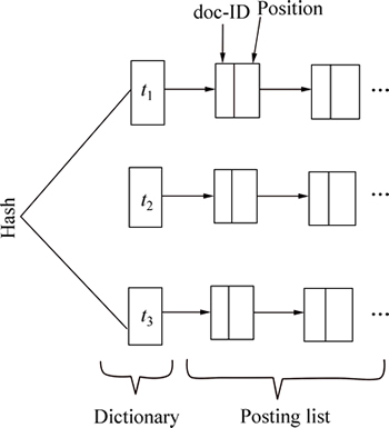
Fig. 1 P.I.I (positional inverted index) architecture in search engines

Fig. 2 A transactional graph database containing two graphs

Fig. 3 Graph storage using P.I.I

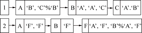
Fig. 4 Each node stored along with its neighbors using P.I.I

3.1 Index construction

General architecture of index construction is pictured in Fig. 5. At first, the input graphs are retrieved from the dataset and then the inverted index tables are built (Fig. 5).

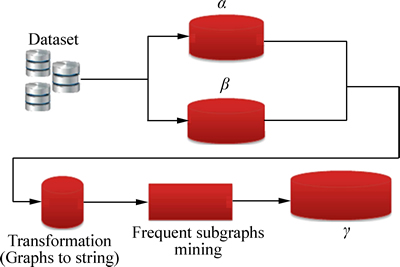
Fig. 5 Index construction architecture

3.1.1 α table construction

To enhance storage and retrieval speed of the graphs, hash table is used. The hash table is generated using the techniques that some of them have been used in No-SQL database (i.e. Column-based techniques). That is to say, when the key/value technique in some of standard hash table fails to solve the problem, the value section is implemented as key/value, which is easier to manage and has higher storage and retrieval pace.

Figure 6 illustrates graph database containing 3 graphs (g₁, g₂, g₃). Using hash table and column-based technique, the three graphs are stored like Table 1.

Fig. 6 Graph database with three graphs

Table 1 α table: An inverted index on edges

Here, the vertexes and the edges are arranged based on lexicographic order. That is to say, the vertexes with lower ASCII codes are set as starting vertex (where an edge is started) and the vertexes with higher ASCII code is set as the end vertex (where an edge is ended). For instance, ‘A’ comes before ‘B’ and ‘B’ comes before ‘C’, which leads to edges AB and BE (instead of BA and EB). Table 1 lists how the graphs are stored.

For instance, Table 1 indicates that edge AB in the graph database occurs in three graphs No. 1, 2 and 3. Graph No. 1 appears between vertexes (1, 2) and (1, 3) and graph No. 2 appears between vertexes (1, 2), (1, 4), (1, 5) and graph No. 3 appears between vertexes (1, 2), (1, 4), (1, 5) (‘%’ is splitter). As another example, CD appears only in graph No. 1 between vertexes (4, 5). It is notable that α table is constructed with reading the database once and there is no further reading the database.

3.1.2 β table construction

When α table is almost full, a set of features can be stored and later used to process the queries. The table is called β, which, like α table, is created based on column-based technique. A graph database is pictured in Fig. 6 and β table is filled as Table 2.

Table 2 β table: An inverted index on nodes

First column “Graph ID” in the table lists the database graphs, i.e. the keys in the original hash table. The columns under “value” are created using column-based technique so that the column “Node” includes vertexes of the graph and column “Neighbor” lists neighbors of each node. For instance, first record of β table shows that in graph 1, one vertex tagged ‘A’, has two neighbors tagged with ‘B’, and two nodes ‘B’ once has neighbors ‘A’ and ‘C’, another has neighbor ‘A’; node ‘C’ has neighbors tagged with ‘B’ and ‘D’; node ‘D’ has neighbor ‘C’ (‘%’ is splitter of neighbor of each node and # is splitter of each neighbor of each node). In Algorithm 1, first part of index construction is shown.

Algorithm 1: BuildIndex1()

Input: Graph dataset D

Output: α and β tables

1 for each graph g_i in D

2   for each edge e_j in g_i

3     if (α contains (e_j))

4       if (α, get(e_j), contains (i))

5         add label of e_j into α

6       else

7         add i and label of e_j into α

8     else

9        add e_j, i and label of e_j into α

10 start_j=get start point of e_j

11 end_j=get end point of e_j

12 if (β contains (i))

13  if (β, get(i), contain (start_j))

14    add end_j to neighbors of start_j

15  else

16    add start_j to β and end_j as neighbor of start_j

17 else

18  add i to β, start_j and end_j as neighbor’s start_j

3.1.3 γ table construction

This table is used to store the frequent subgraphs. Having β and α built, the frequent subgraphs are mined using gSpan algorithm [26]. They are indexed after determining the frequent subgraphs. For a graph with |v| vertexes, time complicacy to find maximum standard labeling form is O(|v|!) as we need to test all possible relations that the nodes could have relation to each other. Therefore, this method is not effective with very large graphs. To improve pace of the process, we can use nodes invariant so that each node is assigned with a feature and isomorphism remains unchanged during mapping process. For instance, isomorphism, level, or vertex label remain unchanged throughout mapping process. The invariant vertex reduces standard labeling computation. The vertex invariants can be used for categorizing the graphs into equal classes. For example, all vertexes in one class have identical vertex invariants. Because of this, standard labeling form can be obtained from the largest or smallest lexicographic order based on the classes and with no need to compute different orders. It is notable that two subgraphs are isomorph when they are classified in the same class, where m represents number of the partitions, which is classified using labeling invariants with vertexes p₁, p₁, p₂, …, p_n, thennumber of different permutations such as   is much less than |V|!. To explain more the labeling process and vertexes degree, here the vertexes are classified into different partitions so that each partition includes the vertex with the same label and degree, and each partition is identified based on the label and degree of the vertexes. Figure 7 illustrates this method; in Fig. 7(a), the vertexes υ₁, υ₀, and υ₃ have the same label as vertex a and only υ₂ is labeled with b. In addition, each edge is labeled with the same label (E) except for the edge between υ₁ and υ₀ that is labeled F. Adjacency matrix of the graph based on lexicographic order is pictured in Fig. 7(b). Based on the level and label, the vertexes can be classified into different groups such as p₀={υ₁}, p₁={υ₀, υ₃} and p₂={υ₂} [27]. The partition p₀ includes vertexes of degree 3, partition p₁ includes two vertexes of degree 1 and label a, and partition p₂ includes vertexes of degree 1 and label b. The classification method is illustrated in Fig. 7(c). The adjacency matrix obtained from the graph is also pictured in Fig. 7. Through this, only 1!×2!×1!=2 permutations are performed. However, number of permutations for a graph with 4 vertexes is 4!=24.

When the frequent subgraphs are converted with a unique string, a hashing table γ is implemented using column-based technique to be used to store frequent subgraphs. That is to say, the table key (i.e. unique string column), value of unique string (upper triangle matrix entries arranged in a column), graph_ids column (graph number) and last column (graph_edges) are used to store the edges of the graph. For instance, the graph illustrated in Fig. 7(a) as a frequent graph is stored in hash table Frequent_Subgraphs as Table 3. Algorithm 2 shows second part of index construction.

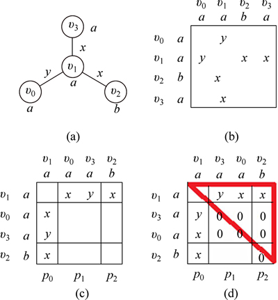
Fig. 7 A graph of size 4(a), adjacency matrix of (a) (b), matrix partitioned according to node degree (c), and permutation of matrix according to minimum lexicography (d)

Table 3 γ table: To store frequent subgraphs

Algorithm 2: BuildIndex2()

Input: Graph dataset D, set of frequent subGraph (FGs) F

Output: γ tables

1  for each f g_i in F

2    cluster nodes according to degree of each node

3    sort clusters according to degree of each cluster

4    for each cluster C_i

5      sort labels of nodes according to lexicographic order

6      put nodes into new cluster with degree and label equal to each other

7    sort new cluster, first according to degree and then nodes labels

8    set adjacency matrix rows according to nodes of new clusters sorted

9    for each sorted cluster containing more than one code

10     calculate all permutations for rows of adjacency matrix

11  for each permutations

12    fill upper triangular matrix

13    calculate string s_p using putting together columns of upper triangle matrix and add to Min[p]

14 calculate minimum lexicographic of Min and put it in key

15 if (γ contains (key))

16   if (γ, get(key) contain (i))

17       add edges of f g_i to γ

18   else

19      add i to γ

20 else

21   add key, i, to γ

3.2 Query processing

General architecture of queries is shown in Fig. 8.

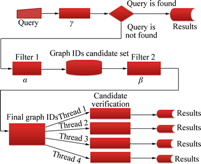
Fig. 8 Query processing architecture

3.2.1 Indexed queries

The queries are coded as unique strings using the vertex invariants technique. Then, the string is sent to γ table as key and the query answer is returned. In Algorithm 3, the case which query is indexed is shown.

Algorithm 3: IfQueryIndexed()

Input: query q and γ table

Output: set of graphs containing q

1 Transform query q as a string according to Lines 1–14 of Algorithm 2 and put it on str

2 If (γ contains (str))

3 Return results

4 else

5 IFQueryNotIndexed()

3.2.2 Non-indexed queries

First, each edge in the query is determined with its frequency. Then, the query space is pruned using the resultant α table. That is to say, each edge is sent to the hash table and its frequency is computed and checked using α table. The graph’s ID of which the number of edges and frequency (number of edges in the query) is identical is returned. Afterward, graphs with the mentioned features which might have no isomorph subgraph are removed using vertexes matching in the query and β table. For instance, even the graphs with one adjacent vertex in the query are removed from candidate answers when no such feature is observed for the subgraphs of the candidate answer set. To improve processing speed, the program is implemented as a multi-threading technique. That is to say, the IDs set that query is processed in them (some graph may be processed more than once for one query) are divided into four threads. As an example, there are 3 threads, when query processing is carried out in 12 graphs, so that each thread, independent from the other threads, processes the query (mining the graphs between some vertexes) and isomorphism test is performed using the vertex invariant [26] (Fig. 8) (Algorithm 4).

Algorithm 4: IFQueryNotIndexed()

Input: query q and, α, β table

Output: set of graphs containing q

1 for each edge e_i in q

2   send e_i into α table and store set of candidate IDs in candidate[i]

3 calculate intersection of candidate[i] and put it in SetCandidate1

4 set Temp=SetCandidate1

5 for each ID_i in SetCandidate1

6   for each node in q

7      calculate frequency of each nodes

8      if (number of node n_i in graph[ID_i] is less than or equal to number of nodes n_i in q)

9          if (!(node n_i has neighbors that q has same neighbor))

10                  remove ID_i from Temp

11     else

12         remove ID_i form Temp

13 for each ID_j in Temp

14     if (graph[ID_j] contains q)

15              add ID_j into Results

4 Evaluation and results

    The results were obtained by executing the proposed and similar methods in a PC with following specifications:

(1) Programming language: Java

(2) Developing environment: Netbeans IDE 6.9

(3) Processor: Inter (R) Core ^TM 2 Due CPU P8600 @2.40 GHz

(4) Memory: 4 GB

(5) Operating system: Microsoft Windows 7 Professional, 64 bit.

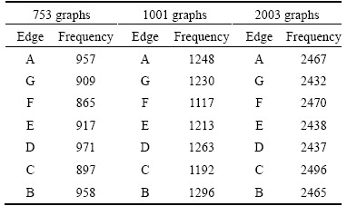
In Table 4 and Table 5, datasets features are listed. The obtained results of index construction time are illustrated in Figs. 9 and 10.

Table 4 Frequency of each edge in graph databases containing 753, 1001 and 2003 graphs

Table 5 Frequency of each node in graph databases containing 753, 1001 and 2003 graphs

Because we use hashing, and column-based techniques and only once scan dataset (these datasets can be shown as edges and ID of each graph), index construction time is decreased, in comparison to FG-index method. But since number of graphs in datasets is increased, index construction time for two method grows. Queries in the following figures are selected randomly with different lengths. Those queries with equal length have different structures. The processing time is based on a dataset including 753 graphs in Fig. 11(b) and a dataset with 1001 graphs in Fig. 11(a). Figures 12 and 13 illustrate the results of queries processed randomly with different lengths on a dataset with 2003 graphs.

Fig. 9 Index construction time on dataset containing 753 graphs

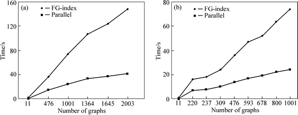
Fig. 10 Index construction time on two dataset containing 2003 (a) and 1001 (b) graphs

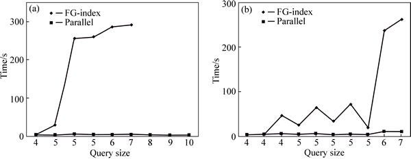
Fig. 11 Query processing on a dataset containing 1001 (a) and 753 (b) graphs

Fig. 12 Query processing time on datasets (a) containing 2003 graphs (b)

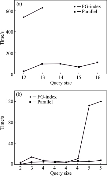
Fig. 13 Query processing time on datasets (a) containing 2003 graphs (b)

5 Conclusion, future works

A graph query processing method was designed to improve response time. The proposed method uses the idea of P.I.I of search engines, hash tables to store and retrieve, and column-based technique for implementation. When the query is part of frequent subgraphs, the answer is obtained without candidate verification; otherwise the query answer is obtained using the filters. Given that graph isomorphism test is one of complicated and time consuming issues, invariant vertexes method was used here. The results from the proposed and similar methods indicate that the proposed method outperforms similar methods regarding processing speed. And some of the future works include capability to be distributed over several systems (tables are independent), and implementation of tables using column-based technique, and finally No-Sql DB all improved graph query processing speed. On the other hand, with ever increase of graph data, there might be cases that the graph database would not be fit in the main memory, in such cases, graph query processing from hard disc (disk-based index) can be carried out. In other words, disc resident inverted index is generated and implemented or specific frameworks such as Hadoop are used. In addition, inverted index can be stored in a distributed form using No-Sql DB and used for graph query processing.

References

[1] CHENG J, KE Y, NG W, LU A. FG-index: Towards verification-free query processing on graph databases [C]// International Conference on Management of Data. Beijing, 2007: 857–872.

[2] BERENDT B, HOTHO A, STUMME G. Semantic web mining [C]// Conference International Semantic Web (ISWC). 2002: 264–278.

[3] MISRA S, BARTHWAL R, OBAIDAT M S. Communication detection in an integrated internet of things and social network architecture [C]// Communication QOS, Reliability and Modeling Syposium. IEEE, 2012: 2787–2805.

[4] WASSERMAN S, IACOBUCCI F. Social network analysis: Methods and applications [M]. Cambridge University Press, 1994.

[5] YAN L, WANG J. Extracting regular behaviors from social media networks [C]// Third International Conference on Multimedia Information Networking and Security. 2011.

[6] CALVIN K. Logic induction of valid behavior specifications for intrusion detection [C]// IEEE Symposium on Security and Privacy (S&P). 2000: 142–155.

[7] HILMI Y, ZAKI M J. Graph indexing for reachability queries [C]// 26th International Conference on Data Engineering Workshops (ICDEW). 2010: 321–324.

[8] XIAOGANG Y, YE T, TAO P, CANFENG C, JIAN M. Semantic-based graph index for mobile photo search [C]// Second International Workshop on Education Technology and Computer Science. 2010: 193–197.

[9] PENG T, WANG W, GONG X, TIAN Y, YANG X. A graph indexing approach for content-based recommendation system [C]// IEEE Second International Conference on Multimedia and Information Technology (MMIT). 2010: 93–97.

[10] YAN Xi-feng, YU S P, HAN J. Graph indexing: A frequent structure-based approach [C]// ACM SIGMOD International Conference on Management of Data (SIGOM). 2004: 335–346.

[11] XU G, ZHANG Y, LI L. Web mining and social networking [M]. Melbourn: Springer, 2010.

[12] IVANCSY, RENATA I, VAJK I. Clustering XML documents using frequent subtrees [J]. Advances in Focused Retrieval, 2009, 3: 436–445.

[13] YUAN J, LI X, MA L. An improved XML document clustering using path features [C]// Fifth International Conference on Fuzzy Systems and Knowledge Discovery. 2008.

[14] RAJARAMAN, ULLMAN J D. Mining of massive datasets [M]. 2nd ed. Cambridge: Cambridge University Press, 2012.

[15] AGGARWAL C, WANG Hai-xun. Managing and mining graph data [M]. Springer, 2010.

[16] HAN J, KAMBER M. Data mining concepts and techniques [M]. USA, Diane Cerra, 2006.

[17] DINARI H, NADERI H. A survry of frequent subgraphs snd subtree mining methods [J]. International Journal of Computer Science and Business Informatics (IJSCBI), 2014, 14(1): 39–57.

[18] HUAN Jun, WANG W, PRINS J. Efficient mining of frequent subgraphs in the presence of isomorphism [C]// Third IEEE International Conference on Data Mining. 2003.

[19] M.KURAMOCHI, KARYPIS G. An efficient algorithm for discovering frequent subgraphs [J]. IEEE Transactions on Knowledge and Data Engineering, 2004, 9: 1038–1054.

[20] ULLMANN J R. An algorithm for subgraph isomorphism [J]. ACM, 1976: 31–42.

[21] SAKR S, PARDEDE E. Graph data management: Techniques and applications [C]// United States of America: Information Science Reference (An Imprint of IGI Global), 2012.

[22] ROSALBA G, SHASHa D. Graphgrep: A fast and universal method for querying graphs [C]// IEEE Proceedings 16th International Conference on Pattern Recognition. 2002: 112–115.

[23] HE Hua-hai, SINGH A K. Closure-tree: An index structure for graph queries [C]// 22nd International Conference on Data Engineering (ICDE’06). 2006: 38–48.

[24] YAN Xi-feng, HAN J. CloseGraph: Mining closed frequent graph patterns [C]// Proceedings of the Ninth ACM SIGKDD International Conference on Knowledge Discovery and Data Mining. 2003: 286–295.

[25] YAN Xi-feng, ZHOU X, HAN J. Mining closed relational graphs with connectivity constraints [C]// ACM SIGKDD International Conference on KNOWLEDGE DISCovery in Data Mining (SIG). 2005: 324–333.

[26] YAN Xi-feng, HAN Jia-wei. Gspan: Graph-based substructure pattern mining [C]// IEEE International Conference on Data Mining (ICDM). 2002: 721–724.

[27] MICHIHIRO K, KARYPIS G. An efficient algorithm for discovering frequent subgraphs [J]. IEEE Transactions on Knowledge and Data Engineering, 2004, 16(9): 1038–1054.

(Edited by YANG Bing)

Received date: 2015-01-04; Accepted date: 2015-04-12

Corresponding author: Hamed Dinari; E-mail: dinari.hamed@yahoo.com, dinari@comp.iust.ac.ir