J. Cent. South Univ. (2017) 24: 448-458

DOI: 10.1007/s11171-017-3447-y

Identification and nonlinear model predictive control of MIMO Hammerstein system with constraints

LI Da-zi(李大字)¹, JIA Yuan-xin(贾元昕)¹, LI Quan-shan(李全善)², JIN Qi-bing(靳其兵)¹

1. Department of Automation, Beijing University of Chemical Technology, Beijing 100029, China;

2. Beijing Century Robust Technology Co. Ltd., Beijing 100020, China

Central South University Press and Springer-Verlag Berlin Heidelberg 2017

Abstract: This work is concerned with identification and nonlinear predictive control method for MIMO Hammerstein systems with constraints. Firstly, an identification method based on steady-state responses and sub-model method is introduced to MIMO Hammerstein system. A modified version of artificial bee colony algorithm is proposed to improve the prediction ability of Hammerstein model. Next, a computationally efficient nonlinear model predictive control algorithm (MGPC) is developed to deal with constrained problem of MIMO system. The identification process and performance of MGPC are shown. Numerical results about a polymerization reactor validate the effectiveness of the proposed method and the comparisons show that MGPC has a better performance than QDMC and basic GPC.

Key words: model predictive control; system identification; constrained systems; Hammerstein model; polymerization reactor; artificial bee colony algorithm

1 Introduction

Identification and control methods of nonlinear MIMO systems are attracting more and more attention in recent years [1, 2]. Linear models and nonlinear models are used to describe nonlinear systems. Nonlinear model is good at representing industrial process because it is capable of describing the global behavior of the process over the whole operating range. What’s more, nonlinear models can often be used to provide better approximations than linear ones [3]. Hammerstein system is one of the most frequently used nonlinear structures [4]. A few of methods have been proposed in recent literatures to identify Hammerstein system, most of which mainly focus on single-input-single-output (SISO) processes [5, 6], while few methods are used to handle multi-input-multi-output (MIMO) problems. In the last decade, artificial neural network (ANN) has been frequently used to approximate nonlinearity [7] in many fields. To reach a satisfied approximation, a large amount of process data are needed to train the neural network, which is impossible for many industrial processes. For identifying the nonlinearity of Hammerstein model, the steady-state responses are used in Ref. [8]. And TANG et al [9] extended this theory to Wiener system. Steady- state response method is effective for identification of static nonlinearity of SISO system, but it cannot be used directly to deal with MIMO processes because of the Inputs-Outputs coupling. In this paper, this method is extended to MIMO Hammerstein systems. Then, an optimization algorithm will be enclosed for identification of the predictive MIMO model.

Many optimization algorithms have been proposed, such as genetic algorithm (GA) [10], particle swarm optimization (PSO) [11]. Artificial bee colony (ABC) algorithm proposed by KARABOGA simulated the foraging behavior of honey bee swarm [12]. The performance of ABC algorithm is competitive to other population-based algorithms such as PSO, GA [13]. However, ABC algorithm also faces some problems such as the local optima when dealing with complex multimodal problems. The reasons focus on the balance between exploration and exploitation which contradict to each other [14]. To achieve the two destinations, a modified ABC algorithm-NABC inspired by the new Luus-Jaakola algorithm (NLJ) [15], is proposed in this paper.

After the model of the nonlinear MIMO plant is estimated, MPC is introduced for the dynamic system control. MPC refers to a class of computer control algorithms which can use a dynamic model to predict future behavior of the systems [16]. The generalized predictive control (GPC), proposed by CLARKE [17] is one of the most widely used model-based control methods [18]. GPC of T-S fuzzy model is presented [19]; the recursive least square technique and the Lagrange Multiplier method are implemented. A multivariable GPC approach is applied for a waste heat recovery process with organic rankine cycle [20]. This community tended to ignore its potential for dealing with constraints. In other words, it points to the fact that, when constraints are ignored, predictive control is equivalent to conventional [21]. In practical control problems, constraints of system have to be usually taken into account. Since constraints may lead to a slow control rate and cannot guarantee the stability of the system [22]. Genetic algorithm is used for optimization in nonlinear predictive control of a SISO first-order process with constraints [23]. LI et al [24] accelerated GA by improving the initial population for the control of solid oxide fuel cells (SOFCs) process. However, it is unable to use this method directly to handle MIMO control problems with constraints. Automatic control of MIMO nonlinear system is still facing some problems such as the stability issues and the complexity [25].

In this work, identification and nonlinear model predictive control of MIMO Hammerstein system with constraints are considered. The identification of MIMO Hammerstein system based on a novel artificial bee colony algorithm is illustrated. A modified generalized predictive control algorithm MGPC is detailed. And a experiment is carried out about a polymerization reactor using the proposed method to show the advancements. Some conclusions are made in the last section.

2 MIMO Hammerstein systems

As shown in Fig. 1, Hammerstein system consists of a static nonlinear block followed by a dynamic linear block. The model of MIMO Hammerstein system can be described as

       (1)

where ξ are system inputs, intermediate signals, outputs and noises respectively; n is the order of the linear transfer function; F(·) is the nonlinear function and A(z^-1), B(z^-1) are parameters of the linear differential equations. The identification target is to estimate A(z^-1),B(z^-1), C(z^-1) and F based on input-output data collection [U, Y] of the system.

Fig. 1 Structure of Hammerstein model

Because of the uncertainty of the intermediate signals X, the linear part cannot be identified directly. In this work, a two-step method is used for identifying the Hammerstein model. The nonlinear static part is identified using steady-state input-output data. In this method: a) accurate estimation of the static nonlinear part is needed to avoid approximation errors so that a high-accuracy optimization algorithm is demanded; b) high accuracy of the nonlinearity assures consistency of parameter estimation of the linear part. Once the nonlinear part of the system is determined, the Sub-model Method (SM) [26] is then applied to identify the dynamic linear part using the input-output data. The identification method of Hammerstein is detailed in the following section.

2.1 Modified artificial bee colony algorithm inspired by NLJ

2.1.1 Brief description of ABC algorithm and NLJ algorithm.

The artificial bee colony algorithm consists of three groups of bees: employed bees, onlookers and scout bees. The initial population of the solutions is generated according to the following equation:

            (2)

where represents the ith food source in the population and n is the population size; i=1, 2, …, SN, j=1, 2, …, n. x_min,j and x_max,j are the lower and upper bounds for dimension j; SN is the number of food sources. Each employed bee X_i generates a new food source V_i=[v_i,1, v_i,2, …, v_i,D] by using the solution search equation:

                      (3)

where both k and j are randomly chosen indexes; D is the number of variables (problem dimension); k is different from i; f_i,j is randomly chosen in the range [-1, 1]. Once a new food source is obtained, the fitness of V_i is calculated. Similar with some other optimization algorithms, a greedy selection mechanism is employed between the old and candidate solutions, where the fitness of V_i will be compared with that of X_i.

In practice, it is necessary for ABC algorithm to keep a balance between the global exploration and local exploitation, easily trapped in “premature” or local optimum sometimes. NLJ algorithm is a stochastic search based optimization algorithm, which can get a very good estimation for any optimization problem with a determined performance as long as the search range and the search density are large enough. For each iteration, p groups of unknown parameter estimates are generated by

                (4)

where a(i) is the ith parameter; j=1, …, p, stands for the groups number; p is the group number of employed bees and k indicates the iteration; rand_ji, i=0, 1, …, n, stands for n+1 numbers randomly generated between 0 and 1.

Then, the current optimal solution can be chosen as the initial value of the next iteration. And the updating forum is:

                (5)

The range of the next search can be updated according to the current optimal solution by Eq. (5).

However, the search range and density of the NLJ algorithm cannot be infinite. Because the search results depend on the initial value of the parameters, NLJ cannot be applied to an optimization problem without prior knowledge.

2.1.2 A higher-accuracy artificial bee colony algorithm- NABC.

The performance of NLJ algorithm depends on the initial value of the parameters, while ABC can be easily trapped in local optima. To keep a good balance between the global exploration and local exploitation, a novel NABC algorithm is proposed. NABC accelerates convergence speed and avoids local optima problem of ABC algorithm.

The modified search equation of ABC algorithm is used which is proposed by GAO and LIU [14], devised as follows:

                   (6)

This search equation increases the exploitation of ABC algorithm which makes it possible that the best solution in current population can be used to improve the convergence performance. After that, the best solution of ABC is used to initialize NLJ algorithm and a better solution can be obtained. The proposed NABC algorithm can be summarized as

Step 1: Find the global optimization and corresponding fitness function value of each bee by using the search equation Eq. (6), where k stands for the iteration and l is the number of groups.

Step 2: Make of the initial value of NLJ algorithm.

Step 3: Get the optimal solution and its fitness function value If then

Step 4: Set k=k+1, and go to Step 1 until the requirements are met.

2.2 Identification of MIMO Hammerstein systems

2.2.1 Identification of the nonlinearity using NABC

According to Eq. (1), the input-output model of the Hammerstein system can be described as

   (7)

where Y(k), U(k) and ξ(k) are n×1 control sequences and white noise at sampling instant k;is a difference operator; △ andare n×n dimensions; i, j=1, …, n, d_ij is delay operator.

The following assumptions are made about the nonlinear system

Assumption 1: The dynamic linear part of the system discussed in this work is square and asymptotically stable. Because the nonlinearity is static, the Hammerstein system is asymptotically stable.

Assumption 2: The input U utilized for identification of the dynamic linear part is a PBRS independent from the noise {ξ(k)}.

Assumption 3: The process {ξ(k)} is a white stochastic process with zero mean and variance σ².

As well known, Assumption 1 implies the existence of the steady-state response for constant inputs of the following system:

                (8)

where Y_s is the step-response of the process. Then, the steady-state responses of system (8) can be described as {y_s(k)}, corresponding to a generic constant input. The structure of the nonlinearity can be approximated by following polynomial:

,

                        (9)

where n is the number of inputs and outputs, are constant parameters of F(·) which need to be identified. Once the steady-state input-output pairs are obtained, the nonlinearity can be identified. The parameters are estimated by minimizing the following fitness function:

                    (10)

where M is the length of the data set and is the estimated value of x_i(k). For any practical problem, an appropriate length of the polynomial can be chosen.

2.2.2 Identification of the linear block

Once the nonlinearity of the Hammerstein is identified, the internal signal X (see Fig. 1) can be obtained. Then, the dynamic linear part of the MIMO system can be described as

           (11)

where X=[x₁, x₂, …, x_r]^T, Y=[y₁, y₂, …, y_r]^T. Then, the MIMO system can be decomposed into r sub-models shown in Fig. 2. And the transfer function can be described as

              (12)

The nonlinearity has been identified in section 2.2.1, and then the internal signal X can be obtained by Eq. (4). The identification problem can be transformed into optimization problems by minimizing the following fitness function:

                          (13)

where i=1, 2, …, r and are prediction outputs. Parameters A_i, D_ij can be obtained through solving the optimization problem by NABC algorithm.

3 MGPC for MIMO Hammerstein system with constraints

3.1 Model predictive control problem formulation

Numerous MPC techniques have been developed over years, but the main idea (i.e. predictive model, receding horizon approach and optimization of a cost function) is always the same. Generally, a set of future control increments is obtained at each sampling instant k

      (14)

where N_u is the control horizon and is the ith predictive control increment at sampling instant k, i=0, 1, …, N_u-1. The control objective is to minimize differences between the predicted outputs and the reference trajectory W(k+j) over the prediction horizon N≥N_u while the excessive control increments are penalized. The cost function is typically used described as

               (15)

where λ(j) is weighting factor. In practice, only the first element of the control increments Eq. (14) determined by Eq. (15) is applied to the process.

                 (16)

At k+1, the next sampling instant, the prediction is moved one step forward and the true output is updated. The whole procedure is repeated as above steps. Considering constraints of the system, the optimization problem which is used to determine future control increments is described as follows:

                    (17)

s.t.

;

;

Fig. 2 Structure decomposition of MIMO system

The predictive output for j=1, …, N is:

where is calculated from the dynamic linear block of the process; D(k) is the unmeasured disturbance which is estimated from

where is calculated from the model and Y(k) is measured.

3.2 Solving constrained problems in MGPC algorithm

The target of MPC is to minimize the cost function (15), that is to say, the optimization problem is typically used described as follows:

            (18)

A Diophantine equation is introduced below which is corresponding to the prediction for

              (19)

where E_j(z^-1) and F_j(z^-1) are unique polynomial vectors of order j-1 and n, respectively; j=1, 2, …, N.

Another Diophantine equation is used to get the step response matrix,

 (20)

G_j and and H_j are vectors of n×n dimensions,

Ignore the noise impact of the future, the j-step prediction result can be acquired as follows:

;

Definethe prediction outputs can be obtained as

    (21)

where are sampling values with n×n dimensions of step response of the system.

Now constraints of control increments △U(k), control values U(k) and output values Y(k) are considered:

;

;

where △U_max, Y_max and △U_min, Y_min are upper limit and lower limit respectively,; is the all ones lower triangular matrix; I is unit matrix; is the step response matrix of the system.

For the MIMO systems with constraints, we can reformulate the optimization problem (17) as the following quadratic programming,

                           (22)

s.t.

where

The MGPC optimization task Eq. (22) may turn into infeasibility problem if the output constraints are considered inevitably, such as the admissible set might result in empty value in the optimization problem. To solve this problem, some slack variables are taken into account. The quadratic programming problem of MPC turns to

     (23)

s.t.

;

;

where ε_min and ε_max are slack variables of length N; ρ_min>0, ρ_max>0 are weights. Let V=[△U^T(k)(ε_max)^T(ε_min)^T]^T be a vector containing all decision variables of MGPC algorithm. The optimization problem (20) can be rewritten in a standard QP form as follows:

                       (24)

s.t.

where

,

;

.

Then, the future control increments △U(k) can be obtained by solving the standard QP and only the first element of the calculated △U(k) is actually applied to the process. It can be seen from Eq. (24) that the nonlinearity of Hammstein system is handled directly during the optimization process and this is the specialization of MGPC compared to general constrained MPC methods.

The control structure of the process is shown in Fig. 3, U(k) are the inputs and Y(k) are the outputs. A Hammerstein model is used to predict outputs W(k) is the reference vector. And the error D(k) is used to correct the predictive output The optimizer carries out the proposed MGPC algorithm. The flow chart of the MGPC algorithm is illustrated in Fig. 4.

The MGPC algorithm can be summarized as follows:

Step 1: Initialization.

Step 2: Identify the transfer function to get the linear model.

Step 3: Solve the Diophantine equation.

Step 4: Solve the QP problem to determine △U(k).

Step 5: Apply

Step 6: Calculate the output Y(k), set k←k+1and go to step 4.

4 MGPC for MIMO Hammerstein system with constraints

A nonlinear MIMO polymerization reactor is considered to illustrate the effectiveness of the proposed method. The structure of the process is shown in Fig. 5. The plant consists of a polymerization solution of methyl-methacrylate (MMA) which is initiated by azo- bis-iso-butotyronitrile (AIBN). The model is based on the standard free-radical reaction kinetic mechanism and under standard assumptions [27]. The manipulated variables are the initiator flow rate stream Fi and the input power Q_c. The controlled variables are the reactor temperature T and the conversion factor x_p. The process description of the system is detailed in Ref. [27] and the loading conditions are listed in Table 1.

4.1 Identification process

4.1.1 Identification of nonlinearity

To perform identification process of the static nonlinear part of the polymerization reactor, a sequence of steady-state inputs are within the range from 0.1 kJ/s to 1.0 kJ/s for the input power (Q_c), and from 9×10^{-9 m3}/s to 11×10^{-9 m3}/s for the initiator flow rate stream (Fi). The sample time is 100 s. The steady-state responses of T and x_p are shown in Figs. 6 and 7, respectively. The relationship between Q_c and T is shown in Fig. 8. It can be seen that it is almost linear and the influence of Fi on T is negligible. So, only the relationship between x_p and Q_c, Fi needs to be identified. Here, T, x_p, Fi and Q_c are defined as y₁, y₂, u₁ and u₂. According to Eq. (9), the relationship between y₂ and u₁, u₂ can be described as

      (25)

And the identification problem can be equivalent to the following optimization problem:

Fig. 3 Control structure of MIMO Hammerstein system with constraints

Fig. 4 Flowchart of proposed method

Fig. 5 Continuous polymerization reactor structure

                   (26)

Table 1 Operating conditions

Fig. 6 Steady-state responses of temperature T in the case of step changes in Q_c and Fi

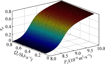
Fig. 7 Steady-state responses of conversion factor x_p in the case of step changes in Q_c and Fi

The proposed NABC algorithm is applied to solve the optimization problem. To avoid blindness and inefficiency of the optimal search, 30 times Monte Carlo experiments are made and the average of these values is taken. The identification result of the nonlinearity is shown in Fig. 9, where the true outputs of the nonlinearity is drawn in solid line and the estimates given by NABC algorithm is in dash line.

4.1.2 Identification of linear block

Considering that the nonlinearity has been estimated in the previous section, the dynamic linear block can be described as

                      (27)

where G₁₁=B₂₁/A₁, G₂₁=B₂₁/A₂, G₂₂=B₂₂/A₂ are the transfer functions. The SM method is performed to identify the parameters. The order of each transfer function is chosen to be 2. Then, the identification problem can be equivalent to the following optimization problems:

                    (28)

                   (29)

where y₁(k), y₂(k) are the true outputs and are the predictive outputs; θ₁=[a₁₁, a₁₂, b₁₁(0), b₁₁(1), b₁₁(2)]^T; θ₂=[a₂₁, a₂₂, b₂₁(0), b₂₁(1), b₂₁(2), b₂₂(0), b₂₂(1), b₂₂(2)]^T.

Fig. 8 Relationship between T and Q_c

Fig. 9 Actual and estimated curves of nonlinearity of conversion factor x_p

The NABC algorithm is performed to search for the parameters of the transform function. Also all the results are the averages of 30 times Monte Carlo experiments. To illustrate the effectiveness of the identification process, a pseudo random signal of length 3000 was applied to the estimation Hammerstein model. Figure 10 indicates the actual curve and the estimated curve of the controlled variable T. The actual and estimated outputs of x_p are illustrated in Fig. 11. The figures reveal that the estimated outputs are mostly the same as the true outputs. Because of the error of the nonlinearity identification, error exits between the identified and true output of x_p. Figure 12 shows the comparison of convergence between NABC and ABC algorithm. The three estimated parts of the Hammerstein model (linear part of T, linear part of x_p and the nonlinear part of x_p) are illustrated in the figure. One can notice that NABC has a faster convergence speed than ABC algorithm. Table 2 shows the value of integral square error (ISE) calculated by the two algorithms, and makes it clear that the accuracy of NABC algorithm is higher than that of ABC algorithm.

Fig. 10 Actual and estimated values of temperature excited by pseudo random signal

Fig. 11 Actual and estimated values of conversion factor x_p excited by a pseudo random signal

4.2 Nonlinear model predictive control by MGPC

In this simulation, the control horizon of MGPC is N_u=4, the predictive horizon is N=4, and the constraints of the system are described as follows

Fig. 12 Convergence of fitness of T (a), linear part (b) and (c) nonlinearity of x_p by NABC; convergence of fitness of T (d), linear part (e) and nonlinearity (f) of x_p by ABC

Table 2 ISE of three parts of Hammerstein system by NABC and ABC

The parameters for the comparative methods are all the same with MGPC.

To illustrate the effectiveness of the MGPC algorithm, comparisons with QDMC [28] and GPC [20] method are made, and the operation conditions are all the same. The references and control result of T and x_p are shown in Figs. 13-14, respectively. The results of QDMC, GPC and MGPC are drawn. It is clear that MGPC reaches the reference trajectory faster thanQDMC and GPC. On top of that, MGPC is much stable than those of the other two methods. Values of manipulated variables calculated by the three algorithms are shown in Figs. 15-16. Because of the nonlinearity, QDMC shows a low rate of change of the manipulated variables because of a large amount of calculation. And GPC cannot handle the constraints well. In order to show these results more clearly, Figs. 17(a), (b) and (c)illustrate the errors between the reference and the controlled value of T by the three different control algorithms. And Figs. 18(a), (b) and (c) indicate the errors of x_p. As one can see from Fig. 18, for control of the conversion factor, MGPC reaches the reference at about 1099 s for the first time, while QDMC at about 1600 s and GPC algorithm at about 1500 s. It shows that the MGPC has a better performance than those of QDMC and GPC.

Fig. 13 Temperature (T) tracking with QDMC, GPC and MGPC control of process

Fig. 14 Convergence factor (x_p) Tracking with QDMC, GPC and MGPC control of process

Fig. 15 Initiator flow rate stream of polymerization reactor calculated by three methods

Fig. 16 Input power of polymerization reactor calculated by three methods

Fig. 17 Temperature error by A: QDMC method; B: GPC method; C: MGPC method

Fig. 18 Conversion factor error by three methods:

5 Conclusion

An identification method and a nonlinear model predictive control algorithm (MGPC) for MIMO Hammerstein system with constraints are proposed. In the identification method, the main point is to estimate the parameters of the static nonlinearity and the dynamic linear part by minimize fitness functions. Therefore, a modified artificial bee colony algorithm which solves the local optima problem of ABC is proposed to search for the optimal solution. In the control algorithm of MIMO Hammerstein system, the difficulty is to deal with the constraints and nonlinearity. The proposed MGPC algorithm transforms the control problem with constraints into a standard QP problem. The optimization problem of MPC can then be solved in one step. MGPC algorithm is more computationally efficient than QDMC algorithm. Simulation studies have shown that the proposed methods have good performance in noise disturbance rejection and set-point tracing under the condition of constraints.

References

[1] BAYRAK A, TATLICIOGLU E. Online time delay identification and control for general classes of nonlinear systems [J]. Transactions of the Institute of Measurement and Control, 2013, 35(6): 808-823.

[2] GARNA T, BOUZRARA K, RAGOT J, MESSAOUD H. Nonlinear system modeling based on bilinear Laguerre orthonormal bases [J]. ISA Transactions, 2013, 52(3): 301-317.

[3] PEARSON R K, POTTMANN M. Gray-box identification of block-oriented nonlinear models [J]. Journal of Process Control, 2000, 10(4): 301-315.

[4] MEHTA U, MAJHI S. Identification of a class of Wiener and Hammerstein-type nonlinear processes with monotonic static gains [J]. ISA Transactions, 2010, 49(4): 501-509.

[5] WANG F, XING K, XU X. Parameter estimation of piecewise Hammerstein systems [J]. Transactions of the Institute of Measurement and Control, 2014: 0142331214531007.

[6] DEMPSEY E J, WESTWICK D T. Identification of Hammerstein models with cubic spline nonlinearities [J]. IEEE Transactions on Biomedical Engineering, 2004, 51(2): 237-245.

[7] SUNG S W. System identification method for Hammerstein processes [J]. Industrial & Engineering Chemistry Research, 2002, 41(17): 4295-4302.

[8] ALONGE F, D'IPPOLITO F, RAIMONDI F M, et al. Identification of nonlinear systems described by Hammerstein models [C]// Decision and Control, 2004. Proceedings. 43rd IEEE Conference on. New York: IEEE, 2004, 4: 3990-3995.

[9] TANG Y, QIAO L, GUAN X. Identification of Wiener model using step signals and particle swarm optimization [J]. Expert Systems with Applications, 2010, 37(4): 3398-3404.

[10] TANG K S, MAN K F, KWONG S, HE Q. Genetic algorithms and their applications [J]. Signal Processing Magazine, IEEE, 1996, 13(6): 22-37.

[11] KENNEDY J. Particle swarm optimization [M]// Encyclopedia of Machine Learning. New York, US: Springer, 2010: 760-766.

[12] KARABOGA D. An idea based on honey bee swarm for numerical optimization [R]. Technical report-tr06, Erciyes University, Engineering faculty, Computer engineering department, 2005.

[13] KARABOGA D, AKAY B. A comparative study of artificial bee colony algorithm [J]. Applied Mathematics and Computation, 2009, 214(1): 108-132.

[14] GAO W, LIU S. A modified artificial bee colony algorithm[J]. Computers & Operations Research, 2012, 39(3): 687-697.

[15] PAN L D. The application of optimization for regulator selftuning online [J]. Journal of Beijing University of Chemical Technology, 1984, 11(1): 17-18. (in Chinese)

[16] CHEN W H, HU X B. A stable model predictive control algorithm without terminal weighting [J]. Transactions of the Institute of Measurement and Control, 2005, 27(2): 119-135.

[17] CLARKE D W. Application of generalized predictive control to industrial processes [J]. Control Systems Magazine, IEEE, 1988, 8(2): 49-55.

[18] OUARI K, REKIOUA T, OUHROUCHE M. Real time simulation of nonlinear generalized predictive control for wind energy conversion system with nonlinear observer [J]. ISA Transactions, 2014, 53(1): 76-84.

[19] JIANG J, LI X, DENG Z, YANG J, ZHANG Y, LI J. Thermal management of an independent steam reformer for a solid oxide fuel cell with constrained generalized predictive control [J]. International Journal of Hydrogen Energy, 2012, 37(17): 12317-12331.

[20] ZHANG J, ZHOU Y, LI Y, HOU G, FANG F. Generalized predictive control applied in waste heat recovery power plants [J]. Applied Energy, 2013, 102: 320-326.

[21] CAMACHO E F, ALBA C B. Model predictive control [M]. New York: Springer Science & Business Media, 2013.

[22] ZHANG L, WANG J, GE Y, WANG B. Constrained distributed model predictive control for state-delayed systems with polytopic uncertainty description [J]. Transactions of the Institute of Measurement and Control, 2014: 0142331214528970.

[23] ONNEN C, R, KAYMAK U, SOUSA J M, VERBRUGGEN H B, ISEMANN R. Genetic algorithms for optimization in predictive control [J]. Control Engineering Practice, 1997, 5(10): 1363-1372.

[24] LI Y, SHEN J, LU J. Constrained model predictive control of a solid oxide fuel cell based on genetic optimization [J]. Journal of Power Sources, 2011, 196(14): 5873-5880.

[25] K, KOCIJAN J. Non-linear model predictive control for models with local information and uncertainties [J]. Transactions of the Institute of Measurement and Control, 2008, 30(5): 371-396.

[26] ZHAO W X, ZHOU T. Weighted least squares based recursive parametric identification for the submodels of a PWARX system [J]. Automatica, 2012, 48(6): 1190-1196.

[27] SOROUSH M, KRAVARIS C. Multivariable nonlinear control of a continuous polymerization reactor [C]// Proceedings of the 1992 merican Control Conference, Chicago, US: IEEE, 1992: 607-614.

[28] DOYLE F J, OGUNNAIKE B A, PEARSON R K. Nonlinear model-based control using second-order Volterra models [J]. Automatica, 1995, 31(5): 697-714.

(Edited by DENG Lü-xiang)

Cite this article as: LI Da-zi, JIA Yuan-xin, LI-Quan-shan, JIN Qi-bing. Identification and nonlinear model predictive control of MIMO Hammerstein system with constraints [J]. Journal of Central South University, 2017, 24(2): 448-458. DOI: 10.1007/s11171-017-3447-y.

Foundation item: Projects(61573052, 61273132) supported by the National Natural Science Foundation of China

Received date: 2015-11-13; Accepted date: 2016-01-13

Corresponding author: LI Da-zi, Professor, PhD; Tel: +86-10-64434930; E-mail: lidz@mail.buct.edu.cn