
Fig. 2 Measurements of ten 2D ultrasonic anemometers (The wind time series are simultaneously recorded with 4 Hz sampling rate during a period of 1 h and each series contains 14400 points)
In order to further test the scaling behavior of non- stationary time series, surrogate time series are generated by shuffling the original wind speed records [2, 3, 23]. The test results show that those new surrogate data preserve the distribution of the original ones, while the corresponding long range correlations are destroyed, as shown in Fig. 3(a). Statistical results in Fig. 3(b) illustrate that the shuffling signals exhibit uncorrelated behavior (H=0.5, i.e., white noise). Abovementioned analysis confirms that the scaling behavior of near-surface wind speed is due to the temporal correlations, rather than the distribution.
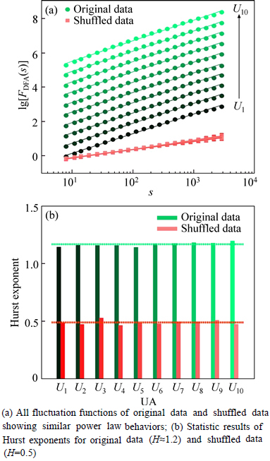
Fig. 3 Results of DFA analysis: (Different gradient colors represent different UAs. The DFA fluctuation functions for original data are vertically shifted for clarity)
4.2 Temporal-spatial cross-correlation analysis using conventional techniques
The wind speed time series are measured simultaneously from the ten 2D UAs deployed in line with 1 m interval as shown in Fig. 2. We set U1 as the reference location. Next, three conventional methods, i.e., Pearson coefficient, cross-correlation function and DCCA are implemented to evaluate the spatial cross-correlation between the U1 and other Ux (U1×Ux, x = 2, 3, …, 10).
4.2.1 Analysis results by Pearson coefficient
The spatial cross-correlation levels between the U1 and other nine Ux (i.e., U1×Ux , x=2, 3, …, 10) using the method of Pearson coefficient are 0.9191, 0.8797, 0.8467, 0.8077, 0.7956, 0.7771, 0.7568, 0.7319, 0.7117, respectively (see Fig. 4). In this figure we can identify that there indeed exist strong spatial cross-correlations between the referenced U1 and other Ux, and the corresponding intensity value increases with a decrease in the intervals. Due to the intrinsic limitation of the Pearson coefficient, this method only provides the global measurement of the level of the spatial cross-correlation. In other words, this analysis cannot reflect the cross- correlation variance as a function of the time scales.
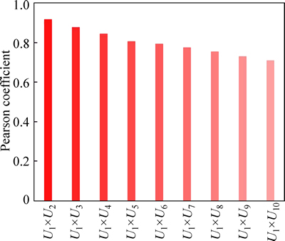
Fig. 4 Test results using Pearson coefficient
4.2.2 Test results by cross-correlation function
Next, cross-correlation function is adopted to evaluate the spatial variability of wind speed data. The highlight of this method is that it is capable of measuring the distinction between two time series as a function of the lag time. This technique can be implemented as the convolution of two series {xi} and {yi}, and the cross-correlation function is calculated as  (i=1, 2, …, N), where
  denotes the complex conjugate of xi, and τ is the lag parameter.
Compared with the standard Pearson coefficient, the superiority of the cross-correlation function is that it concerns about the time lag problem. When τ=0 (no delay), the cross-correlation results agree well with the deployment of UAs. Besides, the cross-correlation levels C(τ) decay with the time lag τ. However, except for τ=0, there is no stable relationship between the intensities of C(τ) and the deployment of UAs, and in most cases, the values of C(τ) for different Ux (x=2, 3, …, 10) vary slightly at the same τ, as shown in Fig. 5.
4.2.3 Analysis results by DCCA method
Concerning about the non-stationary features of the signals, a new strategy, called detrended cross- correlation analysis method (DCCA) was developed to study cross-correlation between time series. Taking into account the fractal and non-stationary characteristics in wind speed data (see Section 4.1), we therefore apply DCCA method to investigate cross-correlations between the U1 and other Ux.
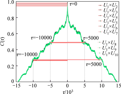
Fig. 5 Test results using cross-correlation function (Except for τ=0, there is no stable relationship between the intensities of C(τ) and deployment of UAs, and in most cases (τ ≠ 0), there is little difference in C(τ) for different UAs, such as τ=-10000, -5000, 5000, 10000)
Figure 6 exhibits DCCA results in log-log scale. Cross-correlations between the U1 and other UAs are all very well fitted by power laws (Fig. 6(a)) with λi=1.1853, 1.1942, 1.2014, 1.1971, 1.2134, 1.2179, 1.2204, 1.2208,1.2306 for U1×Ux(x=2, 3, …, 10), respectively (see Fig. 6(b)). This figure informs us that if we analyze the cross-correlation between the U1 and other Ux utilizing the DCCA method, we have the similar behaviors with little difference. It is obvious that the DCCA method can quantify long-range power-law cross-correlations, while it cannot quantify the level of cross-correlations in function of time scale s.
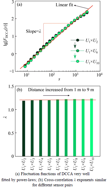
Fig. 6 Cross-correlation results between U1 and other Ux using DCCA technique:
4.3 Test results by DCCA cross- correlation coefficient
In order to overcome the limitation of DCCA, ZEBENDE [14] proposed a novel modified method, i.e., DCCA cross-correlation coefficient which is defined as the ratio between the detrended covariance function and the detrended variance function. The main advantages of this proposed method, compared with the DCCA strategy, is that it can quantify the level of cross-correlation as a function of time scales as well as can easily identify the seasonal components.
Next, the DCCA cross-correlation coefficients are calculated between the U1 and other Ux (see ρDCCA in Fig. 7). The corresponding cross-correlations are always positive and not perfect until s≈1000 (250 s). In most cases, starting from lower levels of cross correlation (ρDCCA≤0.3) at the small time scales (s≤12, i.e., 3 s), they will transfer to perfect cross-correlation (ρDCCA≈1) at large time scales (s≥1000, i.e., 250 s). That is why we cannot use only the DCCA method to quantify the level of cross-correlation.
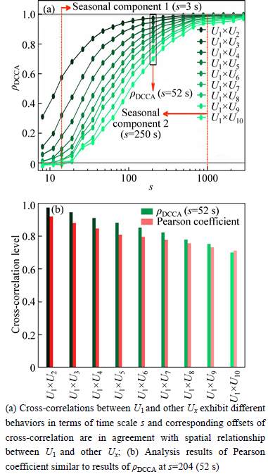
Fig. 7 Results using DCCA cross-correlation coefficient:
In contrast to the results of DCCA, the cross- correlations between the U1 and other Ux exhibit different behaviors in terms of time scale s and in most cases the offsets of cross-correlation for different sensor pairs are in agreement with the spatial arrangement of Ux shown in Fig. 1. In other words, the smaller the distance to U1 is, the larger the cross-correlation there will be at a certain time scale (see Fig. 7(a)). This figure also informs us an important fact that the spatial cross-correlations between the U1 and other UAs change according to the time scale s. These results may have far-reaching consequences for wind field reconstruction and wind forecasting. Moreover, in Fig. 7(a) we can identify the seasonal components, i.e., s=12 (3 s) divides ρDCCA into weak cross-correlation (s<12) or not (s>12), and s=1000 (250 s) divides ρDCCA into perfect cross-correlation (s>1000) or not (s<1000). Finally, compared with the measurement of Pearson coefficient (see Fig. 7(b)), similar results are found at certain time scale (s=204, i.e., 52 s) in Fig. 7(a).
5 Conclusions
1) The temporal-spatial cross-correlation between the time series recorded at different locations has many potential applications. However, tests on ten wind-speed data of anemometers with regular arrangement show that the conventional methods of cross-correlation, such as Pearson coefficient, cross-correlation function and DCCA, are unsuitable to measure the temporal-spatial cross-correlation between the wind speed time series. Pearson coefficient and DCCA are single metric techniques, thus for the cases in which the temporal- spatial cross-correlation changes as the time scale changes, these two methods failed. The cross- correlation results using cross-correlation function are fluctuated in many cases, which are not well matched with the regular arrangement of UAs.
2) Taking into account the non- stationary features of wind speed time series, a state-of- art method, called DCCA cross-correlation coefficient, was applied to analyze the cross-correlation between the different sensor pairs. The experimental results show that this method can accurately quantify the level of cross- correlation between non-stationary wind speed time series and also successfully identify the seasonal component. Next, we plan to use this robust method to do the works of the wind field reconstruction based on real measurement and wind pattern recognition.
References
[1] GOVINDAN R B, KANTZ H. Long-term correlations and multifractality in surface wind speed [J]. Europhysics Letters, 2004, 68(2): 184-190.
[2] KAVASSERI R G, NAGARAJAN R. Evidence of crossover phenomena in wind-speed data [J]. IEEE Transactions on Circuits and Systems, 2004, 51(11): 2255-2262.
[3] KAVASSERI R G, NAGARAJAN R. A multifractal description of wind speed records [J]. Chaos Solitons & Fractals, 2005, 24(1): 165-173.
[4] KOCAK K. Examination of persistence properties of wind speed records using detrended fluctuation analysis [J]. Energy, 2009, 34(11): 1980-1985.
[5] FENG Tao, FU Zun-tao, DENG Xing, MAO Jiang-yu. A brief description to different multi-fractal behaviors of daily wind speed records over China [J]. Physics Letters A, 2009, 373(45): 4134-4141.
[6] TELESCA L, LOVALLO M. Analysis of the time dynamics in wind records by means of multifractal detrended fluctuation analysis and the Fisher-Shannon information plane [J]. Journal of Statistical Mechanics-Theory and Experiment, 2011, 2011(7): 07001.
[7] SANTOS M D O, STOSIC T, STOSIC B D. Long-term correlations in hourly wind speed records in Pernambuco, Brazil [J]. Physica A, 2012, 391: 1546-1552.
[8] ANJOS P S D, SILVA A S A D, STOSIC B, STOSIC T. Long-term correlations and cross-correlations in wind speed and solar radiation temporal series from Fernando de Noronha Island, Brazil [J]. Physica A, 2015, 424: 90-96.
[9] BECK V, DOTZEK N. Reconstruction of near-surface tornado wind fields from forest damage [J]. Journal of Applied Meteorology and Climatology, 2010, 49(7): 1517-1537.
[10] AZAD H B, MEKHILEF S, GANAPATHY V G. Long-term wind speed forecasting and general pattern recognition using neural networks [J]. IEEE Transactions on Sustainable Energy, 2014, 5(2): 546-553.
[11] KRISTOUFEK L. Measuring correlations between non-stationary series with DCCA coefficient [J]. Physica A, 2014, 402: 291-298.
[12] CHEN Yan-guang. A new methodology of spatial cross-correlation analysis [J]. PLOS ONE, 2015, 10(5): 01261585.
[13] PODOBNIK B, STANLEY H E. Detrended cross-correlation analysis: A new method for analyzing two nonstationary time series [J]. Physical Review Letters, 2008, 100(8): 38-71.
[14] ZEBENDE G F. DCCA cross-correlation coefficient: Quantifying level of cross-correlation [J]. Physica A, 2011, 390(4): 614-618.
[15] PENG C K, BULDYREV S V, HAVLIN S, SIMONS M, STANLEY H E, GOLDBERGER A L. Mosaic organization of DNA nucleotides [J]. Physical Review E, 1994, 49(2): 1685-1689.
[16] da SILVA M F, de AREA LEAO PEREIRA E J, dA SILVA FILHO A M, MIRANDA J G V, ZEBENDE G F. Quantifying cross- correlation between Ibovespa and Brazilian blue-chips: The DCCA approach [J]. Physica A, 2015, 424: 124-129.
[17] DONG Ke-qiang, FAN Jie, GAO You. Cross-correlations and structures of aero-engine gas path system based on DCCA coefficient and rooted tree [J]. Fluctuation and Noise Letters, 2015, 2(14): 1550014.
[18] DONG Ke-qiang, GAO You, JING Li-ming. Correlation tests of the engine performance parameter by using the detrended cross- correlation coefficient [J]. Journal of the Korean Physical Society, 2015, 66(4): 539-543.
[19] CAO Guang-xi, HAN Yan. Does the weather affect the Chinese stock markets? Evidence from the analysis of DCCA cross-correlation coefficient [J]. International Journal of Modern Physics B, 2015, 29(01): 14502361.
[20] SHEN Chen-hua, LI Chao-ling, SI Ya-li. A detrended cross-correlation analysis of meteorological and API data in Nanjing, China [J]. Physica A, 2015, 419: 417-428.
[21] PODOBNIK B, JIANG Zhi-qiang, ZHOU Wei-xing, STALEY H E. Statistical tests for power-law cross-correlated processes [J]. Physical Review E, 2011, 84: 066118.
[22] KRISTOUFEK L. Power-law correlations in finance-related Google searches, and their cross-correlations with volatility and traded volume: Evidence from the Dow Jones Industrial components [J]. Physica A, 2015, 428: 194-205.
[23] IVANOV P C, AMARAL L, GOLDBERGER A L, HAVLIN S, ROSENBLUM M G, STRUZIKLL Z R, STANLEY H E. Multifractality in human heartbeat dynamics [J]. Nature, 1999, 399(6735): 461-465.
(Edited by YANG Hua)
Cite this article as: ZENG Ming, LI Jing-hai, MENG Qing-hao, ZHANG Xiao-nei. Temporal-spatial cross-correlation analysis of non-stationary near-surface wind speed time series [J]. Journal of Central South University, 2017, 24(3): 692-698. DOI: 10.1007/s11771-017-3470-4.
Foundation item: Projects(61271321, 61573253, 61401303) supported by the National Natural Science Foundation of China; Project(14ZCZDSF00025) supported by Tianjin Key Technology Research and Development Program, China; Project(13JCYBJC17500) supported by Tianjin Natural Science Foundation, China; Project(20120032110068) supported by Doctoral Fund of Ministry of Education of China
Received date: 2015-11-03; Accepted date: 2016-12-01
Corresponding author: ZENG Ming, Associate Professor, PhD; Tel: +86-13114806460; E-mail: zengming@tju.edu.cn


 Central South University Press and Springer-Verlag Berlin Heidelberg 2017
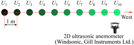
 and
and  k=1, 2, …, N, where
  and
and denote the global average of {xi} and {yi}. Then, two profiles are divided into N-s overlapping boxes with equal length s, each starting at i and ending at i+s, in other words, each containing s+1 values. For both time series, in the v-th box that starts at i and ends at i+s, we define the “local trend”
  and
and  (i≤k≤i+s, v=1, 2, …, N-s) to be the ordinate of a linear least-squares fit. The “detrended walk” comes to be the difference between the original walk and the local trend. The detrended covariance of the residuals in each box isdefined as
 Next, we calculate the DCCA covariance function by averaging
  over all overlapping N-s boxes of size s,
 (1)
(1) (2)
(2) versus lg[s]. Supposing {xi}={yi}, the detrended covariance
 reduces to the detrended variance
  used in the DFA method. In this case, the exponent is equivalent to the well-known Hurst exponent H, which takes values between 0 and 1 for stationary processes, while takes 1
 (3)
(3)