J. Cent. South Univ. Technol. (2009) 16: 0690-0696

DOI: 10.1007/s11771-009-0114-3

Short-term forecasting optimization algorithms for wind speed along Qinghai-Tibet railway based on different intelligent modeling theories

LIU Hui(刘 辉)^{1, 2}, TIAN Hong-qi(田红旗)^{1, 2}, LI Yan-fei(李燕飞)^{1, 2}

(1. Key Laboratory of Traffic Safety on Track, Ministry of Education, Central South University,

Changsha 410075, China;

2. School of Traffic and Transportation Engineering, Central South University, Changsha 410075, China)

Abstract: To protect trains against strong cross-wind along Qinghai-Tibet railway, a strong wind speed monitoring and warning system was developed. And to obtain high-precision wind speed short-term forecasting values for the system to make more accurate scheduling decision, two optimization algorithms were proposed. Using them to make calculative examples for actual wind speed time series from the 18th meteorological station, the results show that: the optimization algorithm based on wavelet analysis method and improved time series analysis method can attain high-precision multi-step forecasting values, the mean relative errors of one-step, three-step, five-step and ten-step forecasting are only 0.30%, 0.75%, 1.15% and 1.65%, respectively. The optimization algorithm based on wavelet analysis method and Kalman time series analysis method can obtain high-precision one-step forecasting values, the mean relative error of one-step forecasting is reduced by 61.67% to 0.115%. The two optimization algorithms both maintain the modeling simple character, and can attain prediction explicit equations after modeling calculation.

Key words: train safety; wind speed forecasting; wavelet analysis; time series analysis; Kalman filter; optimization algorithm

1 Introduction

Many Chinese scholars have studied the effects of strong cross-wind on trains in recent years, and attained some breakthrough research results [1-5]. Similar research has also been made in some railway developed countries [6-10]. The research results show that to safeguard running trains which are susceptible to the effects of extreme cross-wind along railway, building a strong wind speed monitoring and warning system is an feasible option. Along Qinghai-Tibet railway, extremely strong cross-wind happens frequently. Historical maximum wind speed exceeds 40 m/s, which makes a potential threat for running trains’ safety. To protect trains against the strong cross-wind, Chinese scholars have developed a strong wind speed monitoring and warning system [1-5]. For this system, one of core technologies is to build high-precision short-term wind speed prediction models.

In wind power domain, wind speed forecasting can be classified as short-term, medium-term and long-term forecasting [11]. Short-term forecasting is to build models and calculate forecasting values less than 10 h. Medium-term forecasting is to build models and calculate forecasting values between 10 and 24 h. Long-term forecasting is to build models and calculate forecasting values more than 24 h [12]. The forecasting algorithms usually include neural networks, time series analysis, Kalman filtering, genetic algorithm, wavelet analysis, etc [11-20]. Compared with other relatively steady time series, such as power load series [17-18] and traffic flow series [19-20], wind speed time series is more unsteady and harder to attain high-precision multi-step forecasting values.

With the trains’ running velocity improved gradually, the wind speed short-term forecasting for train safety has become a new research focus. The wind speed forecasting just started in China several years ago [12-16]. The main existing problems are the low forecasting accuracy and limited forecasting steps. Aiming at those problems, we proposed two optimization algorithms.

2 Forecasting precision requirement of strong wind speed monitoring and warning system

(1) The models should be capable of making high-precision forecasting at least 1 min ahead for wind speed series measured by each meteorological station.

(2) The models should be as simple as possible to allow fast verification and obviously reduce modeling calculation time.

(3) Each model has the corresponding forecast equation, which is easy for wide application and optimization research.

3 Framework of two optimization algorithms

The framework of the two proposed optimization algorithms is illustrated in Fig.1, which includes five main steps.

The detailed steps are described as follows, where t is the sampling time, n is the wavelet decomposition layer, and k is the ahead forecasting step.

(1) Use wavelet analysis method to make decomposition and reconstruction calculation for the original wind speed series {v(t)} (t=1, 2, 3, …), then obtain the high-frequency wind speed series {vⁿ(t)} (t=1, 2, 3, …; n=1, 2, 3, …) and the low-frequency wind speed series {w(t)} (t=1, 2, 3, …).

(2) Use improved time series analysis method to build prediction models for series {vⁿ(t)} (t=1, 2, 3, …; n=1, 2, 3, …) and {w(t)} (t=1, 2, 3, …), then calculate the k-step ahead forecasting values  (t=1, 2, 3, …; n=1, 2, 3, …; k=1, 2, 3, …) and  (t=1, 2, 3, …; k=1, 2, 3, …).

(3) Use Kalman time series analysis method to build prediction models for series {vⁿ(t)} (t=1, 2, 3, …; n=1, 2, 3, …) and {w(t)} (t=1, 2, 3, …), then calculate the one-step ahead forecasting values  (t=1, 2, 3, …; n=1, 2, 3, …) and  (t=1, 2, 3, …).

(4) Make weighted computations for the k-step ahead forecasting values  (t=1, 2, 3, …; n=1, 2, 3, …; k=1, 2, 3, …) and  (t=1, 2, 3, …; k=1, 2, 3, …) attained by step (2), then obtain the final k-step forecasting value (t=1, 2, 3, …; k=1, 2, 3, …) for original series v(t).

(5) Make weighted computations for the one-step ahead forecasting values  (t=1, 2, 3, …; n=1, 2, 3, …) and (t=1, 2, 3, …) attained by step (3), then obtain the final one-step forecasting value  (t=1, 2, 3, …) for original wind speed series v(t).

4 Modeling process of optimization algorithm based on wavelet analysis method and improved time series analysis method

To verify the performance of proposed algorithms, we used the actual wind speed data measured by the 18th meteorological station along Qinghai-Tibet railway to make simulation calculation. The former 1st-150th data were used to establish models, the later 151st-200th data to inspect forecasting precision.

4.1 Decomposition and reconstruction calculation of original wind speed series

Select Daubechies6 wavelet to decompose original wind speed series {v(t)}. Decomposition layer was n=3. Use Mallat algorithm to reconstruct wind speed series {vⁿ(t)} and {w(t)} in different scales. The curve of series {v(t)} is shown in Fig.2.

{vⁿ(t)} (n=1, 2, 3) was the 1st to 3rd layer high-frequency wind speed series. {w(t)} was the 3rd layer low-frequency wind speed series. To facilitate modeling, {v¹(t)} was renamed as {X_4t}, {v²(t)} was renamed as {X_3t}, {v³(t)} was renamed as {X_2t}, and {w(t)} was renamed as {X_1t} series.

4.2 Modeling steps of improved time series analysis method

As the decomposed wind speed series was relatively steady, we selected improved time series analysis method to build the corresponding prediction models.

Taking three-step ahead forecasting for example, the modeling steps of improved time series analysis method were described as follows.

(1) Use Box-Jenkins scheme of traditional time series analysis method to build models, select AIC (Akaike information criterion) to determine appropriate model orders, and select moment-estimation algorithm to calculate prediction models’ equation parameters. Based on the calculation results of the upper steps, we finally determined that the optimization model kind for series {X_1t} was ARIMA (6, 1, 0). The corresponding model equation was as follows:

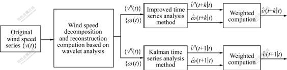
Fig.1 Modeling procedure of optimization algorithm

Fig.2 Curve of original wind speed series {v(t)}

          (1)

Then use Eqn.(1) to calculate the one-step ahead forecasting value for X_lt(200), and the forecasting value was recorded as.

(2) Retain the model kind identified by step (1), re-estimate the model’s equation parameters by series {X_1t(2), X_1t(3), …, X_lt(200),, and attain the new model (Eqn.(2)) that includes the wind speed character of the latest forecasting value . Calculate the one-step ahead forecasting value again by series {X_1t(2), X_1t(3), …, X_lt(200), and attain the two-step ahead forecasting value  for X_lt(200). The updated model equation was as follows:

         (2)

(3) Re-estimate equation parameters by series {X_1t(3), X_1t(4), …, X_lt(200), , and attain the new model (Eqn.(3)) that includes the wind speed character of forecasting values  and. Calculate the one-step ahead forecast value again by {X_1t(3), X_1t(4), …,  and attain the three-step ahead forecasting valuefor X_lt(200). The updated model equation was as follows:

          (3)

 (4) After completing the upper calculation steps, use the latest actually measured wind speed series {X_1t(2), X_1t(3), …, X_lt(201)} to begin a new calculation cycle. For example, calculate the new one-step ahead forecasting value for X_1t(201), successively, finally obtain the three-step ahead forecasting value .

4.3 Weighted computation for each layer forecasting results

Referring to the modeling steps (1)-(4) in Section 4.2, we established prediction models for each layer wind speed series respectively, and made the one-step, three-step, five-step and ten-step ahead forecasting calculation for the later 151st-200th data in each layer.

Then we made weighted computation for each layer forecasting results, and attained the final one-step, three-step, five-step and ten-step ahead forecasting results for the original wind speed series {v(t)}.

The weighted computation equation is shown in Eqn.(4), and the weighted coefficients are ρ₁=ρ₂=ρ₃=1. The computation results are shown in Fig.3.

                  (4)

To reflect the outstanding performance of optimization algorithm based on improved time series analysis method and wavelet analysis method, we used traditional time series analysis method to build prediction models, and made the one-step, three-step, five-step and ten-step ahead forecasting calculation for the same section of the original wind speed series. The forecasting results are shown in Fig.4.

4.4 Forecasting results analysis

International general evaluation indexes were introduced to estimate the upper forecasting precision. The indexes results are shown in Table 1. The evaluation indexes formulas are as follows:

(1) Mean error:         (5)

(2) Mean absolute error:  (6)

(3) Mean relative error: (7)

(4) Mean square error: (8)

From Table 1, we can get that the proposed optimization algorithm based on improved time series

Fig.3 Forecasting results by wavelet analysis method and improved time series analysis method: (a) One-step; (b) Three-step; (c) Five-step; (d) Ten-step

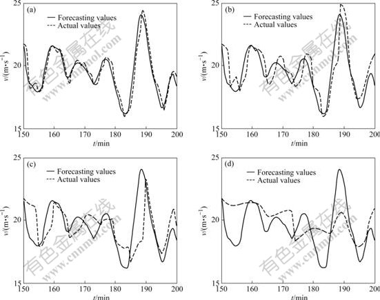
Fig.4 Forecasting results by traditional time series analysis method: (a) One-step; (b) Three-step; (c) Five-step; (d) Ten-step

Table 1 Comparison of forecasting results of optimized algorithm and traditional algorithm

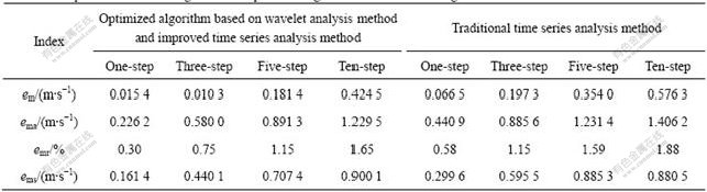
analysis method and wavelet analysis method has excellent algorithm performance, the mean relative errors of one-step, three-step, five-step and ten-step ahead forecasting are only 0.30%, 0.75%, 1.15% and 1.65% respectively, which far exceed the corresponding forecast accuracy of traditional time series analysis method. Besides, this optimization algorithm has good track ability for mutation and jumping wind speed data in multi-step ahead calculation. When the forecasting accuracy is not required so high, using time series analysis method to establish prediction models is also an ideal choice.

Compared Fig.3 with Fig.4 respectively, we can get that the prediction wind speed curve obtained by this optimization algorithm is almost the same as the actual curve, and the prediction curve by traditional time series analysis method appears the delayed phenomena.

5 Modeling process of optimization algorithm based on wavelet analysis method and Kalman filter method

To further improve the one-step ahead forecasting accuracy attained by the optimization algorithm based on improved time series analysis method and wavelet analysis method, we proposed a new optimization algorithm based on wavelet analysis method and Kalman filter method to re-build prediction models, and re-calculated the one-step ahead forecasting values.

5.1 Kalman recursive equations of Kalman filter method

In signal processing domain, the discrete time series system can be described as follows [11]:

          (9)

             (10)

where  X(t) is state vector, Z(t) is observation vector, w(t) is state noise vector, v(t) is observation noise vector, Φ(t+1, t) is state transition matrix, Γ(t+1, t) is motivation transition matrix, and H(t+1) is forecasting output matrix. Eqn.(9) is the state equation, and Eqn.(10) is the observation equation.

The main calculation contents of Kalman filter method are to deduce the right state and observation equations, and to value parameters of Kalman recursive equations [12].

5.2 Modeling calculation steps

The main modeling steps of the new proposed algorithm were described as follows.

(1) Referring to Section 4.1, use wavelet analysis method to accomplish the decomposition and reconstruction calculation for the original wind speed series {v(t)}.

(2) Different from Section 4.1, use time series analysis method to obtain the suitable prediction model equations for each layer wind speed series.

(3) Deduce the state and observation equations by the upper model equations, and then value parameters of Kalman recursive equations.

(4) Use Kalman recursive equations of Kalman filter method to make one-step ahead forecasting calculation for each layer series, and then make weighted computations to attain the final one-step ahead forecasting for the original wind speed series {v(t)}.

Take series {X_1t} for example to illustrate the calculation process of step (3) in Section 5.2.

Supposing that we have obtained Eqn.(1), and X₁(1)=X_1t(t), X₂(t)=X_1t(t+1), …, X₇(t)=X_1t(t+6), Eqn.(1) can be transformed as follows:

          (11)

then

               (12)

Because X₂(t)=X₁(t+1), X₃(t)=X₂(t+1), …, X₇(t)= X₆(t+1), we attained the state equation as follows:

                        (13)

Because Z(t+1)= H(t+1)X(t+1)+v(t+1) (v(t+1) can be supposed as the white noise series), then attained the observation equation as follows [11]:

  (14)

Compared Eqns.(13) and (14) with Eqns.(9) and (10) respectively, we determined the coefficient matrix of state and observation equation. Besides, the other initial values of Kalman recursive equations were determined as follows: X(0│0)=[0], P(0│0)=10I, R(t)=[1] (t=1, 2,  3, …), Q(t)=[1] (t=1, 2 , 3, …).

Then we attained the one-step ahead forecasting calculation for series {v(t)}. The results are shown in Fig.5.

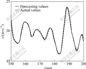
Fig.5 One-step ahead forecasting results by wavelet analysis method and Kalman time series analysis method

5.3 Forecasting results and analysis

Using Eqns.(5)-(8) to estimate the one-step ahead forecasting results by this optimization algorithm, indexes results are shown in Table 2. From Table 2, we can get that the proposed optimization algorithm based on wavelet analysis method and Kalman filter method has obviously improved the one-step ahead forecasting accuracy. Compared Fig.5 with Fig.3(a), we can also find that the tracking ability of optimization algorithm based on wavelet analysis method and Kalman filter method is better than optimization algorithm based on wavelet analysis method and improved time series analysis method.

Table 2 Optimized one-step ahead forecasting results by wavelet analysis method and Kalman time series analysis method

6 Conclusions

(1) The proposed optimization algorithm based on wavelet analysis method and improved time series analysis method can solve the problems of short-term multi-step forecasting for wind speed. It can obtain high-accuracy multi-step ahead prediction results. In addition, this algorithm is suitable for mutation wind speed data and jumping wind speed data, and its tracking ability is excellent.

(2) The proposed optimization algorithm based on wavelet analysis method and Kalman filter method can further improve the one-step ahead forecasting precision. It is especially suitable for the situation that one-step ahead forecasting precision is required to be high.

(3) The two optimization algorithms have all used in Qinghai-Tibet railway strong wind speed monitoring and warning system. These optimization algorithms are compared with other algorithms. The results indicate they do not significantly increase the difficulty of modeling, but significantly improve the model forecasting accuracy.

(4) Based on the Matlab/VB/VC software, each modeling step of the optimization algorithms can be encapsulated as COM components for engineers. With high performance computers, the forecasting output values of the optimization algorithms can completely meet the real-time requirement of monitoring and warning system.

References

[1] TIAN Hong-qi, MIAO Xiu-juan, GAO Guang-jun. Aerodynamic performance of sidewall shape of boxcar under strong crosswind [J]. Journal of Traffic and Transportation Engineering, 2006, 6(3): 5-8. (in Chinese)

[2] ZHOU Dan, TIAN Hong-qi, YANG Ming-zhi, LU Zhai-jun. Comparison of aerodynamic performance of different kinds of wagons running on embankment of the Qinghai-Tibet Railway under strong cross-wind [J]. Journal of the China Railway Society, 2007, 29(5): 32-36. (in Chinese)

[3] TIAN Hong-qi. Study evolvement of train aerodynamics in China [J]. Journal of Traffic and Transportation Engineering, 2006, 6(1): 1-9. (in Chinese)

[4] GAO Guang-jun, TIAN Hong-qi, YAO Song, LIU Tang-hong, BI Guang-hong. Effect of strong cross-wind on the stability of trains running on the Lanzhou-Xinjiang railway line [J]. Journal of the China Railway Society, 2004, 26(4): 36-40. (in Chinese)

[5] LI Yan-fei, LIANG Xi-feng, GAO Guang-jun, LIU Tang-hong. Influence of cross-wind on aerodynamic performances of high-speed container flat car running on embankment [J]. Journal of Railway Science and Engineering, 2007, 4(5): 78-82. (in Chinese)

[6] SUZUKI M, TANEMOTO K, MAEDA T. Aerodynamic characteristics of train/vehicles under cross winds [J]. Journal of Wind Engineering and Industrial Aerodynamics, 2003, 91(1): 209-218.

[7] BARCALA M, MESEGUER J. An experimental study of the influence of parapets on the aerodynamic loads under cross wind on a two-dimensional model of a railway vehicle on a bridge [J]. Journal of Rail and Rapid Transit, 2007, 221(4): 487-494.

[8] HOPPMANN U, KOENIG S, TIELKES T, MATSCHKE G. A short-term strong wind prediction model for railway application: Design and verification [J]. Journal of Wind Engineering and Industrial Aerodynamics, 2002, 90(10): 1127-1134.

[9] IMAI T, FUJII T, TANEMOTO K, SHIMAMURA T, MAEDA T, ISHIDA H, HIBINO Y. New train regulation method based on wind direction and velocity of natural wind against strong winds [J]. Journal of Wind Engineering and Industrial Aerodynamics, 2002, 90(12/15): 1601-1610.

[10] ANDERSSON E, HAGGSTROM J, SIMA M, STICHEL S. Assessment of train-overturning risk due to strong cross-winds [J]. Journal of Rail and Rapid Transit, 2004, 218(3): 213-223

[11] PAN Di-fu, LIU Hui, LI Yan-fei. A wind forecasting optimization model for wind farms based on time series analysis and Kalman filter algorithm [J]. Power System Technology, 2008, 32(7): 82-86. (in Chinese)

[12] SANZ S, PEREZ A, ORTIZ E, PORTILLA A, PRIETO L, PAREDES D, CORREOSO F. Short-term wind speed prediction by hybridizing global and mesoscale forecasting models with artificial neural networks [C]// Proceedings of the 8th International Conference on Hybrid Intelligent Systems. Piscataway: Institute of Electrical and Electronics Engineers Computer Society, 2008: 608-612．

[13] TORRES J, GARCIA A, DEBLAS M, DEFRANCISCO A. Forecast of hourly average wind speed with ARMA models in Navarre (Spain) [J]. Solar Energy, 2005, 71(1): 65-77.

[14] LOUKA P, GALANIS G, SIEBERT N, KARINIOTAKIS G, KATSAFADOS P, PYTHAROULIS I, KALLOS G. Improvements in wind speed forecasts for wind power prediction purposes using Kalman filtering [J]. Journal of Wind Engineering and Industrial Aerodynamics, 2008, 96(12): 2348-2362.

[15] ERASMO C, WILFRIDO R. Short term wind speed forecasting in La Venta, Oaxaca, Mexico, using artificial neural networks [J]. Renewable Energy, 2008, 34(1): 274-278.

[16] FERREIRA A, LUDERMIR T, AQUINO D, RONALDO R, LIRA M, NETO N. Investigating the use of reservoir computing for forecasting the hourly wind speed in short-term [C]// Proceedings of the International Joint Conference on Neural Networks. Piscataway: Institute of Electrical and Electronics Engineers Inc, 2008: 1649-1656.

[17] COSTAA A, CRESOPB A, NAVARROA J, LIZCANOC G, MADSEND H, FEITOSAE E. A review on the young history of the wind power short-term prediction [J]. Renewable and Sustainable Energy Reviews, 2008, 12(6): 1725-1744.

[18] MARCIUKAITIS M, KATINAS V, KAVALIAUSKAS A. Wind power usage and prediction prospects in Lithuania [J]. Renewable and Sustainable Energy Reviews, 2008, 12(1): 265-277.

[19] CASTRONETO M, JEONG Y S, JEONG M K, HAN L D. Online-SVR for short-term traffic flow prediction under typical and atypical traffic conditions [J]. Expert Systems with Applications, 2009, 36(3): 6164-6173.

[20] XUE Jie-ni, SHI Zhong-ke. Short-time traffic flow prediction based on chaos time series theory [J]. Journal of Transportation Systems Engineering and Information Technology, 2008, 8(5): 68-72.

(Edited by YANG You-ping)

Foundation item: Project(2006BAC07B03) supported by the National Key Technology R & D Program of China; Project(2006G040-A) supported by the Foundation of the Science and Technology Section of Ministry of Railway: Project(2008yb044) supported by the Foundation of Excellent Doctoral Dissertation of Central South University

Received date: 2008-12-20; Accepted date: 2009-02-26

Corresponding author: LIU Hui, Doctoral candidate; Tel: +86-13107428620; E-mail: liuhui8302@yahoo.com.