J. Cent. South Univ. Technol. (2007)04-0528-09

DOI: 10.1007/s11771-007-0103-3

ACS algorithm-based adaptive fuzzy PID controller and its application to CIP-I intelligent leg

TAN Guan-zheng(谭冠政), DOU Hong-quan(窦红权)

(School of Information Science and Engineering, Central South University, Changsha 410083, China)

_________________________________________________________________________________

Abstract: Based on the ant colony system (ACS) algorithm and fuzzy logic control, a new design method for optimal fuzzy PID controller was proposed. In this method, the ACS algorithm was used to optimize the input/output scaling factors of fuzzy PID controller to generate the optimal fuzzy control rules and optimal real-time control action on a given controlled object. The designed controller, called the Fuzzy–ACS PID controller, was used to control the CIP-I intelligent leg. The simulation experiments demonstrate that this controller has good control performance. Compared with other three optimal PID controllers designed respectively by using the differential evolution algorithm, the real-coded genetic algorithm, and the simulated annealing, it was verified that the Fuzzy–ACS PID controller has better control performance. Furthermore, the simulation results also verify that the proposed ACS algorithm has quick convergence speed, small solution variation, good dynamic convergence behavior, and high computation efficiency in searching for the optimal input/output scaling factors. 

Key words: PID controller; fuzzy control; ACS algorithm; optimal control; input/output scaling factors   

_________________________________________________________________________________

1 Introduction

The proportional-integral-derivative (PID) controller has been widely used to control various industrial objects because of its simple structure, better robustness, and high reliability. Now, around the 90% of industrial objects are controlled by PID controllers. However, the performance of a PID controller fully depends on the tuning of its gain parameters. About this problem, many researchers conducted research^[1-2]. With the development of artificial intelligence, recently many new methods has been used to design PID controllers, such as the differential evolution (DE) algorithm^[3], genetic algorithm(GA)^[4-6], simulated annealing(SA) algorithm^[4], and fuzzy logic control^[6-8]. In these methods, the fuzzy logic control has a good control effect especially for the objects with nonlinear and/or uncertain properties or the objects whose models are very difficult to be established accurately.

For many existing fuzzy PID controllers, basically their control rules came from the experiences of the experts in the related domains and would be easily affected by the subjectivity of the experts. So, for many control systems with highly nonlinear property and stochastic disturbances, the larger error may occur between the ideal rules and the rules from the experts. The selections of the membership functions also have the similar problem. In addition, presently another important problem for fuzzy PID controller is lack of a very efficient and universal design method that is widely suitable to various kinds of objects. Although some researchers studied this problem using GAs^[6] and the optimization algorithm^[7] and obtained valuable results, their methods have some uncertainties in solution quality and control effect. 

The ACS algorithm is an improvement on the ant system (AS) algorithm^[9], the first generation of ant algorithm. Compared with the AS algorithm, the ACS algorithm is more robust, faster, and has a higher probability in obtaining the globally optimal solution. Up to now, the ACS algorithm has been used successfully to solve many practical optimization problems such as the traveling salesman problem^[10], the optimal navigation of mobile robots^[11], the planning of primary distribution circuits^[12].

This paper focused on the efficient and universal design method for the optimal fuzzy PID controller. The ACS algorithm was used to optimize the input/output scaling factors of the controller to generate the optimal fuzzy control rules and implement the optimal fuzzy PID control on a given object.

The basic idea of a fuzzy PID controller is to use the fuzzy control rules to adjust the PID controller gain parameters on line so that the output of the control system has the desired performance.

2.1 PID control law

The expression of PID control law for a continuous system is given as

   (1)

where  e(t) is the error between the input and the output of the system; u (t) is the control action generated by the PID controller; K_p is the proportional gain; T_i is the integral time constant; and T_d is the derivative time constant. In the discrete-time domain, the PID control law can be expressed as

  (2)

where  K_i = K_pT/T_i, K_d = K_pT_d /T, and T is the sampling period; K_p, K_i, and K_d are three adjustable parameters, designing a PID controller means determining the values of these parameters. In this paper, the three parameters are expressed in the following incremental forms: 

            (3)

where  K_p0, K_i0, and K_d0 are the initial PID controller parameters and can be determined using the classical Ziegler-Nichols tuning formula ^[1].

2.2 Structure of fuzzy PID controller

Fig.1 gives the structure of a typical fuzzy PID controller, where r is the input of the system; e is the error of the system; e_c is the time derivative of e; K_p, K_i, and K_d are the outputs of the fuzzy inference mechanism; u is the control action generated by the PID controller; and y is the output of the system. In designing this kind of PID controller, first we need to find out the fuzzy relationships between K_p, K_i, K_d and e, e_c, i.e. determine the fuzzy control rules.

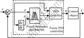
Fig.1 Structure of a typical fuzzy PID controller

When the controller works, in every sampling period, the fuzzy inference mechanism examines the variations of e and e_c and makes on-line adjustment for the parameters K_p, K_i, K_d using the fuzzy control rules so that the PID controller can always generate the optimal control action on the given control object.

E and E_C are used to denote the fuzzy variables of e and e_c respectively; DK_pf, DK_if, DK_df denote the fuzzy variables of the increments DK_p, DK_i, DK_d. The fuzzy sets of E, E_C, DK_pf, DK_if, and DK_df are all selected as {NB, NM, NS, ZO, PS, PM, PB}, where NB, NM, NS, ZO, PS, PM, and PB represent negative big, negative medium, negative small, zero, positive small, positive medium, and positive big, respectively. The fuzzy discourse domains of E, E_C, DK_pf, DK_if, and DK_df are all defined as {-6, -5, -4, -3, -2, -1, 0, +1, +2, +3, +4, +5, +6}. Fig.2 shows the membership functions for E, E_C, DK_pf, DK_if, and DK_df, where m represents the membership.

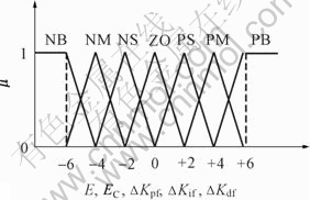
Fig.2 Membership functions for E, E_C, DK_pf, DK_if, and DK_df

2.3 Establishment of fuzzy control rules

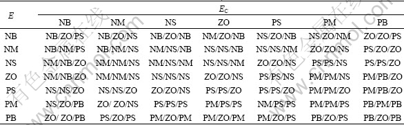
K_p, K_i and K_d have a crucial effect on the performance of PID controller. In general, they should be adjusted in real time according to the system error e and its time derivative e_c. Considering the variation ranges of these parameters in most practical applications, we summarize the variation rules of DK_pf, DK_if and DK_df with E and E_C, i.e. the fuzzy control rules, as shown in Table 1.

Table 1 Control rules of variations of DK_pf /DK_if /DK_df with E and E_C

2.4 Effects of input/output scaling factors on system output

The fuzzy inference mechanism shown in Fig.1 is a two-dimensional fuzzy controller, which has two inputs and three outputs. Assume that during the kth sampling period, the values of the system error e(k) and its variation rate e_c(k) can be quantified according to the following formulas:

 E(k)=INT[G_e×e(k)]              (4)

E_C(k)=INT[G_ec×e_c(k)]           (5)

where  G_e and G_ec are the two input scaling factors of the fuzzy inference mechanism, INT represents the integer function that transforms G_e×e(k) or G_ec×e_c(k) into an integer using the rounding rule. According to the values of E(k) and E_C(k), their fuzzy linguistic values E and E_C can be obtained from Fig.2, and then the fuzzy increments DK_pf, DK_if, and DK_df can be determined from Table 1.

Through defuzzifying DK_pf, DK_if, and DK_df and introducing three coefficients G_p, G_i, and G_d, formula (3) can be rewritten as 

        (6)

where  D[x] means the defuzzification for the fuzzy quantity x using the centroid method; the coefficients G_p, G_i and G_d are the three output scaling factors of the fuzzy inference mechanism. 

Factors G_e, G_ec, G_p, G_i, and G_d are very important parameters of the fuzzy PID controller, and adjusting these factors is a very effective measure to implement the optimal fuzzy control. Hereinafter, we take the adjustment of G_e as an example to explain how to achieve the goal of changing control effect by adjusting the input scaling factors and the output scaling factors.    

Fig.3(a) shows an initial membership function of the error E, which is denoted by E_initial. The input scaling factor G_e corresponding to E_initial is G_e=1. Now, we change the value of G_e, for example, setting G_e=2/3, then the membership function of the error E is changed as: E=G_e­×E_initial = (2/3)×E_initial, as shown in Fig.3(b). As can be seen, if G_e is changed, the fuzzy discourse domain of E is also changed. Assume that in the two cases, the fuzzy linguistic value of E_C maintains the same value ZO. For the point X₁ in Fig.3(a), the fuzzy linguistic value of E is PM, by looking up Table 1 we obtain the fuzzy control rule as:

IF E is PM and E_C is ZO,then DK_pf /DK_if /DK_df is PM/PS/PS.

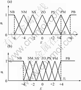
Fig.3 Variation of membership function of E before(a) and after(b) G_e is changed

But, for the point X₁ in Fig.3(b), the fuzzy linguistic value of E is PB, by looking up Table 1 the fuzzy control

rule can be determined as:

IF E is PB and E_C is ZO, then DK_pf /DK_if /DK_df is PM/ZO/PM.

From the two control rules, it can be found that adjusting G_e has an effect on the output of the fuzzy inference mechanism. Adjusting the input scaling factor G_ec also generates the similar effect.

As can be seen from formula (6), after DK_pf, DK_if and DK_df are determined, K_p, K_i, and K_d can still be changed through adjusting the factors G_p, G_i and G_d.

From the above description, we can see that through adjusting the input and output scaling factors G_e, G_ec, G_p, G_i and G_d, we can change the values of K_p, K_i and K_d. This is a very effective measure for changing the control effect. For a given control object, as long as we find the

optimal values of G_e, G_ec, G_p, G_i and G_d, we can implement the optimal control on it.   

3.1 Description of optimization problem

For the fuzzy PID control system shown in Fig.1, the following ITAE criterion can be used to evaluate its control performance:

            (7)

By taking the ITAE criterion as the objective function and the input/output scaling factors G_e, G_ec, G_p, G_i, G_d as the optimized variables, the optimization problem can be described as: for the fuzzy PID control system shown in Fig.1, after the controlled object is given, the task is to find the optimal input/output scaling factors G_e^*, G_ec^* and G_p^*, G_i^*, G_d^* so that the ITAE criterion has the minimum value.

3.2 Generating method of ant moving paths

When using the ACS algorithm to solve an optimization problem, the first step is designing a moving environment for the ants. For the optimized variables G_e, G_ec, G_p, G_i, and G_d, we assume that the value of each of them has five valid digits. According to the ranges of their values in most fuzzy PID controllers, we assume that in their five digits there are two digits before decimal point and three digits after decimal point. In order to use the ACS algorithm conveniently, we express the values of G_e, G_ec, G_p, G_i, and G_d on plane O-xy. As shown in Fig.4, first we draw 25 lines L₁, L₂, …, L₂₅ on plane O-xy, which have equal height and equal interval and are perpendicular to axis x. L₁-L₅, L₆-L₁₀, L₁₁-L₁₅, L ₁₆-L₂₀, and L₂₁- L₂₅ denote the first digit to the fifth digit of G_e, G_ec, G_p, G_i, and G_d, respectively. Then, we divide equally each of these lines into nine segments and thus 10 nodes are generated on each line. The y coordinates of the 10 nodes on each line are 0, 1, …, 9, respectively, which are 10 possible values of each digit.

Fig.4 Diagram for generating nodes and paths

Fig.4 is a grid graph on which there are 25×10 nodes in total. We use n_ij to denote the node j on line L_i. The y coordinate of the node n_ij is denoted by y_ij.

Let an ant depart from the origin O. In its each step forward, it chooses a node from the next line L_i (i=1, 2, …, 25) and then moves to this node along the straight line. When it moves to a node on line L₂₅, it completes one tour. Its moving path can be expressed as Path={O, n_1j, n_2j, ?, n_25j}. Obviously, the values of G_e, G_ec, G_p, G_i, and G_d represented by this path can be computed by the following formulas:

(8)

Fig.4 shows a moving path of an ant. The values of the input and output scaling factors corresponding to the path can be computed as: G_e = 61.478, G_ec =54.267, G_p=34.250, G _i=69.735, and G_d =16.438.

3.3 Selection of nodes on a moving path

For an ant colony, assume that from any node on line L_i to any node on the next line L_i+1, every ant has the same moving time. So, if all ants depart from the origin O at the same time, they will arrive on the terminal line L₂₅ at the same time too.

Let τ_ij (t) denote the pheromone concentration of node n_ij, where t is the iteration counter of the ACS algorithm. Assume that at t = 0 all of the nodes have the same initial pheromone concentration t₀. Assume that the total number of ants is m. In moving process, for an ant k, when it locates on line L_i-1, it will choose a node j from the next line L_i to move to according to the following random transition rule ^[10]:

(9)

where  A represents the set, {0, 1, 2, …, 9}; is the pheromone concentration of node n_iu; η_iu represents the visibility of node n_iu and is computed by the following formula (10); β is a parameter that controls the relative importance of η_iu versus τ_iu(t); q is a random variable uniformly distributed over [0, 1]; q₀ is a tunable parameter (0≤q₀≤1); and J is a node selected according to the following probability formula ^[10] and roulette wheel selection method ^[11]:

       (10)

For the visibilityof node n_ij, we define it as

            (11)

where the values of y_ij^* are set in the following way. In the first iteration of the ACS algorithm, the values of y_ij^* are set respectively to the y coordinates of the 25 nodes corresponding to the initial values of G_e, G_ec, G_p, G_i and G_d, and the initial values of these factors are all set to 1; in each of the following iterations, the values of y_ij^* are set respectively to the y coordinates of the 25 nodes corresponding to the optimal ant path generated by the ACS algorithm in the previous iteration.

3.4 Updating rules of pheromone concentration

3.4.1 Global updating rule

In the ACS algorithm, after each iteration, the pheromone concentration of each node on the best ant tour T* generated since the beginning of the experiment needs to be updated using the following global updating rule ^[10]. The ants therefore are encouraged to search for the paths in the vicinity of T ^*.

τ_ij(t)←(1-ρ)?τ_ij(t)+ρ?Δτ_ij(t)        (12)

where  n_ij is a node belonging to T ^*; (0＜ρ＜1) is pheromone decay parameter; and Δτ_ij(t) is computed by:

Δτ_ij(t)=1/ITAE*              (13)

where  ITAE^* is the value of ITAE criterion corresponding to path T^*.

3.4.2 Local updating rule

In order to expand the search range so that other potential good solutions can emerge, when an ant k passes through a node n_ij, the pheromone concentration of node n_ij needs to be updated immediately using the following local updating rule ^[10]:

τ_ij(t)←(1-ρ)?τ_ij(t)+ρ?τ₀           (14)

If a node is visited for many times by the ants, repeatedly applying the local updating rule will make its pheromone concentration diminish. This has the effect of favoring the exploration of not yet visited nodes.

3.5 Searching algorithm for optimal input/output scaling factors

The ACS algorithm for searching the optimal input/output scaling factors is summarized as follows.

Step 1: Determine K_p0, K_i0 and K_d0 using the classical Ziegler-Nichols tuning formula.  

Step 2: Specify the values of β, q₀, ρ, t₀ and m; Define the maximum number of iterations N_C; For each ant k (k=1, 2, …, m), define a one-dimensional array Path_k with 25 elements, in which the y coordinates of the 25 nodes that ant k will pass through on the grid graph Fig.4 in each iteration of the ACS algorithm will be stored in order. Array Path_k can be used to denote the moving path of ant k.

Step 3: Set the iteration counter t=1 and then place all of the m ants at the origin O.

Step 4: Set i=1.

Step 5: Set k=1.

Step 6: Select a node on line L_i for ant k using formulas (9)-(11), move ant k to the node, and save the y coordinate of the node into the ith element of Path_k; Then, update the pheromone concentration of this node using the local updating rule.

Step 7: Set k?k+1. If k≤m, go to Step 6; Otherwise, continue.

Step 8: Set i?i+1. If i≤25, go to Step 5; Otherwise, continue.

Step 9: For each ant k (k=1, 2, …, m): (a) according to Path_k, compute G_e^k, G_ec^k, G_p^k, G_i^k, and G_d^k using formula (8); (b) Given a unit step signal as the input of the system, perform a simulation experiment using G_e^k, G_ec^k, G_p^k, G_i^k, and G_d^k, and then compute the ITAE value of the system which is denoted by ITAE^k.

Step 10: Compare all of the obtained ITAE values and find the optimal ant path  in the current iteration t. Compare with T ^*, the optimal ant path generated from the beginning of the experiment till the previous iteration t-1 (for the first iteration, directly denote its optimal ant path by T ^*), and denote the new optimal ant path by T ^*, then save the ITAE value and the input/output scaling factors corresponding to path T ^* into ITAE ^* and {G_e^*, G_ec^*, G_p^*, G_i^*, G_d^*}, respectively.

Step 11: Set each element of Path_k to zero, k=1, 2, ?, m.

Step 12: Update the pheromone concentration of each node on path using the global updating rule.

Step 13: Set t?t +1. If t< N_C and all of the m ants do not make the same tour, place all the ants at the origin O and go to Step 4; if t< N_C but all of the m ants make the same tour or t = N_C, output the optimal ant path and its corresponding optimal input/output scaling factors {G_e^*, G_ec^*, G_p^*, G_i^*, G_d^*}, then stop.

4 Motion control of CIP-I leg using proposed fuzzy PID controller

The proposed fuzzy PID controller is called the Fuzzy-ACS PID controller. In order to demonstrate its control performance, this controller is used to control the motion of the CIP-I leg, an intelligent leg prosthesis designed by the authors. CIP-I leg consists of a knee joint, a shank, and a foot. Among them, the knee joint is the most important component that includes a walking speed sensor, an air cylinder with a small D.C. motor, a microprocessor MSP430F149, and batteries. The walking speed sensor is used to measure the walking speed of the leg in real time. The air cylinder is the actuating device used to control the flexion and extension movements of the knee joint. The motor is used to control the opening of a throttle valve in the cylinder. Regulating the opening can change the flexion and extension speeds of the knee joint and thus achieve the goal of changing the walking speed of the leg. The microprocessor controls the motion of the motor according to the measured walking speed. The power of the system is supplied with two small-size rechargeable lithium batteries. CIP-I leg is shown in Fig.5.

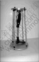
Fig.5 Photo of CIP-I leg

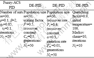
To evaluate the performance of the Fuzzy-ACS PID controller, as the comparison objects, other three typical evolutionary algorithms, including the differential evolution (DE) algorithm^[3], real-coded genetic algorithm (GA)^[4], and simulated annealing (SA) algorithm^[4], are also used to design the optimal PID controller, and the designed PID controllers are called the DE-PID, GA-PID, and SA-PID controller, respectively. The parameter settings of the four algorithms are shown in Table 2.

Table 2 Parameter settings of four evolutionary algorithms

The four PID controllers are used to control the motor of the CIP-I leg. The transfer function of the motor system is G (s) = 6 068/[s (s²+110s +6 068)]. Fig.6 shows the unit step responses of the motor control system. Fig.7 shows the motion simulation result of the CIP-I leg using the Fuzzy-ACS PID controller.

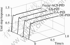
Fig.6 Unit step response of motor control system  using four PID controllers

Fig.7 Swinging motion simulation of CIP-I leg using Fuzzy-ACS PID controller

Table 3 shows the transient-state and stead-state performance indexes of the four PID control systems, including the overshoot M_p, rise time t_r, setting time t_s, stead-state error e_ss and ITAE value. 

Table 3 Performance comparison of four PID controllers

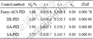
As can be seen from Table 3, the Fuzzy-ACS PID controller has the minimum overshoot, rise time, setting time, and ITAE value compared with other three PID controllers, which means that the Fuzzy-ACS PID controller has better control performance.

The optimal input and output scaling factors corresponding to the motor system obtained from the proposed ACS algorithm, are G_e=2.540, G_ec=93.362, G_p=1.421, G_i=0.000 and G_d=0.231.

5 Performance of proposed ACS algorithm 

5.1 Convergence speed

A simulation experiment was performed on the motor control system using the Fuzzy-ACS PID controller. Fig.8 shows the optimal ITAE value convergence process of the system when using the ACS algorithm to search for the optimal input/output scaling factors. Obviously, its convergence speed is very fast. As can be seen, the optimal solution can be obtained within 10 iterations.

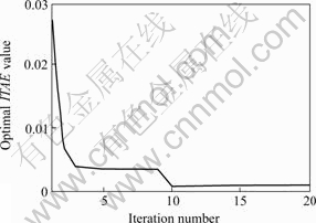
Fig.8 Convergence tendency of optimal ITAE value in an experiment

5.2    Solution variation characteristic

100 simulation experiments were performed on the motor control system using the Fuzzy-ACS PID controller, the result is shown in Fig.9, which reflects the variation of the optimal ITAE value of the control system in 100 experiments. As can be seen, the variation range of the optimal ITAE value is quite small when repeatedly running the ACS algorithm for many times, which means that the solutions generated by the ACS algorithm have good centrality.

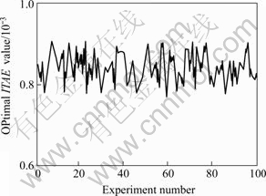
Fig.9 Variation characteristic in optimal ITAE value in 100 experiments

5.3    Dynamic convergence behavior

In order to observe the dynamic convergence behavior of the ACS algorithm during its evolutionary process, two statistic indexes were also adopted in the simulation program, that is, the mean value μ and the standard deviation s. They are defined as follows:

            (15)

       (16)

where  ITAE^k  represents the solution generated by ant k and m denotes the total number of ants; μ denotes the average value of the solutions generated by all ants after the ACS algorithm completes an iteration. The smaller the m value, the better the solution generated by every ant. So, m reflects the accuracy of the algorithm, s represents the centrality of all the solutions. The smaller the s value, the better the centrality of the solutions. So, s reflects the convergence speed of the algorithm.

When using the ACS algorithm to control the motor system of the CIP-I leg, in the process of the algorithm evolution, we recorded the mean value m and the standard deviation s of each iteration. Figs.10 and 11 show the convergence processes of m and s. As can be seen: 1) the mean value m becomes very stable after around 10 iterations, which means that the ACS algorithm has high accuracy and very fast convergence speed; 2) the variation range of the standard deviation s is very small, which means that all the solutions generated by the ACS algorithm in each iteration have good centrality.

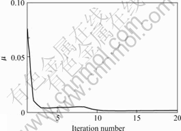
Fig.10 Convergence tendency of mean value (μ) using ACS algorithm

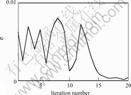
Fig.11 Convergence tendency of standard deviation (σ) using ACS algorithm

5.4 Comparison of computation efficiency of four algorithms

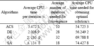
Table 4 presents the computation efficiency comparison of the four evolutionary algorithms. For each algorithm, 100 experiments were performed. In the simulation experiments, we used a computer with 1.7 GHz CPU and 256 MB RAM, and the operating system is the Windows XP. As can be seen from the table, although the ACS needs more CPU time for completing an iteration, because its average number of iterations needed for convergence is the smallest in the four algorithms, its average CPU time needed for obtaining the globally optimal solution is also the smallest in the four algorithms.

Table 4 Comparison of computation efficiency of  four algorithms

A new design method for the optimal fuzzy PID controller was presented. Using this method includes two steps. The first step is determining the optimal input/output scaling factors G_e^*, G_ec^* G_p^*, G_i^* and G_d^* corresponding to the given controlled object using the proposed ACS algorithm. The second step is using the conventional fuzzy control method to implement on-line fuzzy PID control on the given object. The results of the simulation experiments on the motor control system of the CIP-I leg demonstrate that the proposed Fuzzy–ACS PID controller has better transient-state and stead-state performance compared with the DE-PID, GA-PID, and SA-PID controllers. In addition, the simulation results also verify that the ACS algorithm has quick convergence speed, small solution variation, good dynamic convergence behavior and higher computation efficiency in searching for the optimal input/output scaling factors.

[1] ZIEGLER J G., NICHOLS N B. Optimum settings for automatic controllers[J]. ASME Transactions, 1942(65): 433-444.

[2] HO W K, HANG C C, CAO L S. Tuning of PID controllers based on gain and phase margin in specifications[C]// GOODWIN G C, EVANS R J. The 12th IFAC World Congress. Sydney: IFAC, 1993: 267-270.

[3] CHENG S L, HWANG C. Designing PID controllers with a minimum IAE criterion by a differential evolution algorithm[J]. Chemical Engineering Communications, 1998, 170(1): 83-115.

[4] KWOK D P, SHENG F. Genetic algorithm and simulated annealing for optimal robot arm PID control[C]// FOGEL D B. The First IEEE Conference on Evolutionary Computation. Orlando: IEEE, 1994: 707-713.

[5] KROHLING R A, REY J P. Design of optimal disturbance rejection PID controllers using genetic algorithms[J]. IEEE Transactions on Evolutionary Computation, 2001, 5(1): 78-82.

[6] SOUKKOU A, KHELLAF A, LEULMI S. Genetic training of a fuzzy PID[C]// GENTO A M. The International Conference on Modelling and Simulation (ICMS’04). Valladolid, Spain: AMSE, 2004: 185-186.

[7] XU Jing-wei, FENG Xin. Design of adaptive fuzzy PID tuner using optimization method[C]// The Fifth World Congress on Intelligent Control and Automation. Hangzhou, China: Zhejiang University, IEEE Society of Robotics and Automation, 2004: 2454-2458. (in Chinese)

[8] ANZALONE A, IQLESIAS E, GARCIA Y, et al. A fuzzy logic controller with fuzzy scaling factor calculator applied to a nonlinear chemical process[J]. Revista Tecnica de la Facultad de Ingenieria Universidad del Zulia, 2003, 26(3): 189-196.

[9] DORIGO M, BONABEAU E, THERAULAZ G.. Ant algorithms and stigmergy[J]. Future Generation Computer Systems, 2000, 16(8): 851-871.

[10] DORIGO M, GAMBARDELLA L M. Ant colony system: A cooperative learning approach to the traveling salesman problem[J]. IEEE Transactions on Evolutionary Computation, 1997, 1(1): 53-66.

[11] TAN Guan-zheng, HE Huan, SLOMAN A. Global optimal path planning for mobile robots based on improved Dijkstra algorithm and ant system algorithm[J]. Journal of Central South University of Technology, 2006, 13(1): 80-86.

[12] G?MEZ J F, KHODR H M, de OLIVEIRA P M, et al. Ant colony system algorithm for the planning of primary distribution circuits[J]. IEEE Transactions on Power Systems, 2004, 5(2): 996-1004.

___________________________

Foundation item: Project(50275150) supported by the National Natural Science Foundation of China; Project(20040533035) supported by the National Research Foundation for the Doctoral Program of Higher Education of China; Project(05JJ40128) supported by the Natural Science Foundation of Hunan Province, China

Received date: 2006-08-24; Accepted date: 2006-10-27

Corresponding author: TAN Guan-zheng, PhD, Professor; Tel:+86-731-8716259; E-mail: tgz@mail.csu.edu.cn

(Edited by YANG Hua)