J. Cent. South Univ. (2018) 25: 185-195

DOI: https://doi.org/10.1007/s11771-018-3728-5

Numerical investigation of temperature gradient-induced thermal stress for steel–concrete composite bridge deck in suspension bridges

WANG Da(王达)¹, DENG Yang(邓扬)², LIU Yong-ming(刘永明)³, LIU Yang(刘扬)¹

1. School of Civil Engineering, Changsha University of Science & Technology, Changsha 410114, China;

2. Beijing Advanced Innovation Center for Future Urban Design, Beijing University of Civil Engineering and Architecture, Beijing 100044, China;

3. School for Engineering of Matter, Transport & Energy, Arizona State University, 501 E. Tyler Mall,AZ 85281, USA

Central South University Press and Springer-Verlag GmbH Germany, part of Springer Nature 2018

Abstract: A 3D finite element model (FEM) with realistic field measurements of temperature distributions is proposed to investigate the thermal stress variation in the steel–concrete composite bridge deck system. First, a brief literature review indicates that traditional thermal stress calculation in suspension bridges is based on the 2D plane structure with simplified temperature profiles on bridges. Thus, a 3D FEM is proposed for accurate stress analysis. The focus is on the incorporation of full field arbitrary temperature profile for the stress analysis. Following this, the effect of realistic temperature distribution on the structure is investigated in detail and an example using field measurements of Aizhai Bridge is integrated with the proposed 3D FEM model. Parametric studies are used to illustrate the effect of different parameters on the thermal stress distribution in the bridge structure. Next, the discussion and comparison of the proposed methodology and simplified calculation method in the standard is given. The calculation difference and their potential impact on the structure are shown in detail. Finally, some conclusions and recommendations for future bridge analysis and design are given based on the proposed study.

Key words: suspension bridge; steel–concrete composite bridge deck; vertical temperature gradient; finite element method; thermal stress

Cite this article as: WANG Da, DENG Yang, LIU Yong-ming, LIU Yang. Numerical investigation of temperature gradient-induced thermal stress for steel-concrete composite bridge deck in suspension bridges [J]. Journal of Central South University, 2018, 25(1): 185–195. DOI: https://doi.org/10.1007/s11771-018-3728-5.

1 Introduction

Nonuniform temperature distribution in the long-span suspension bridge can be caused by solar radiation, air scattering, and ground reflection [1], which will introduce complex thermal stress within the bridge structure. Steel–concrete composition deck has been widely used in the long span bridges due to its good rigidity and strength. The different thermal conductivities of concrete and steel make the temperature variation more significant than that in other systems. Recently, experiments and field investigations also showed that variable temperature conditions have a more significant effect on the structural behavior than that exerted by operational loads [2–6].

DING et al [7] demonstrated that the temperature at the top of the bridge deck can reach 70 °C in summer. The vertical temperature gradient along the stiffening girder section is nearly 40 °C, which has been considered in the current codes and specifications [7–12]. XIA et al [13] showed that the temperature effects may result in structural damage. With the development of structural health monitoring technology, the field monitoring temperature can be acquired and used in the calculations, which can compensate for the deficiencies in the current codes for temperature effects [14]. The traditional calculation method (TCM) and considering surface curvature effect method (CSCEM) [9], suggested by the current code in China, are two widely used methods for steel–concrete composite structure temperature analysis [15]. A two-dimensional model is usually adopted to describe the temperature distribution of a bridge section [9, 16], which is suitable for simple structures but does not meet the accuracy requirement for large complex structures, such as the steel–concrete composite bridge deck system. Furthermore, the steel–concrete bridge deck is different from other types of bridge deck systems and is sensitive to temperature.

Based on the above, the existing analysis methodologies usually focused on the simplified 2D analysis using specified temperature distribution from codes. The proposed study focuses on the 3D analysis using realistic measured temperature distribution along the entire structure. Thus, more accurate and representative results can be obtained, in principle. The special focus of the proposed study is the investigation of the calculation difference between the classical methods and the proposed framework. The proposed 3D finite element model with realistic temperature field is presented first. Next, the proposed methodology is applied for Aizhai Bridge for demonstration with field measurements. Following this, discussions based on the simulations results are given. Finally, some conclusions and suggestion for future design and analysis are given based on the proposed investigation.

2 Proposed 3D FEM for thermal stress analysis

FEM has been developed since the 1970s [17–21]. The finite difference heat flow models have also been employed to determine the temperature distribution on bridge members [22]. In this study, FEM is proposed for coupled thermal- structural analysis, which is based on numerical integration and not limited by the element shape. Given that the random position in a unit is (x, y, z), the temperature can be expressed as T(x, y, z), as shown in Figure 1.

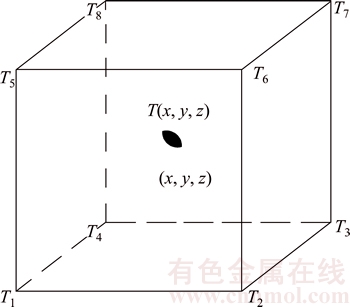
Figure 1 Unit temperature model

The node temperature T(x, y, z) can be expressed as Eq. (1) with the a generic function f(x):

T(x, y, z)=f (T₁, …, T₈)                     (1)

The internal temperature of the structure can be represented as

[T]=[N][T]^e                                               (2)

where [T] is the matrix of the structure temperature; [N] is the matrix of shape function; [T]^e is the matrix of the element temperature.

For the composite structure exposed in the atmosphere, the relationship between the higher temperature T and the lower temperature T_d can be expressed as

   (3)

where n is the direction of the concrete surface normal; β is the heat transfer coefficient; T is the higher temperature; T_d is the lower temperature; λ is the coefficient of heat conductivity of material. The values of l_x, l_y, and l_z are the cosine functions along the x, y, and z directions, respectively.

According to the variational principle, the fonctionelle of temperature can be obtained as follows:

                 (4)

Equation (4) can be expressed as the sum of each fonctionelle of the unit:

                           (5)

where is the fonctionelle of the unit.

The local maximum value for Eq. (5) is obtained when

                     (6)

The following can be deduced by substituting Eqs. (2) and (4) into Eq. (6):

         (7)

where

     (8)

Combining Eqs. (7) and (8), one can have

 (9)

Equation (9) can be written as

                       (10)

The stiffness matrix equation of the temperature for structure can be deduced by Eq. (10), such that

                           (11)

where {P_T}^e is the nodal load of the unit caused by temperature, and {P_T} is the nodal loads of the structure caused by temperature. The internal force and displacement can be obtained by solving Eq. (11).

3 Demonstration and application example

3.1 Bridge description and FEM structural modeling

3.1.1 Bridge description

The Aizhai Bridge is a long-span suspension bridge located in southwestern China. The bridge crosses a 335 m deep U-valley with a main span of 1176 m, as shown in Figure 2. The steel–concrete composite bridge deck, two-way and four-lane, has a clear width of 24 m.

The cross section of the deck module consists of a steel truss beam and a steel–concrete deck system, as shown in Figures 3(a) and (b). The steel– concrete deck system consists of the horizontal I-shaped steel beam, prefabricated bridge deck, and concrete of the overlapped seam cast in place.

3.1.2 FEM structural modeling

A three-segment FEM model consisting of 21120 nodes and 17368 elements is built in the ANSYS program, as shown in Figure 4.

In the model, the element beam188 was taken as the steel stiffer girder and the I-shaped steel beam, and the element solid90 was taken as concrete. To simulate the hinge connection between the stiffen girder and the suspension bar, the boundary conditions at the points of suspension were processed to the linear displacement constraints along the x, y, and z directions, and at the corners the model were processed to the linear displacement constraints along the x and y directions, as shown in Figure 4.

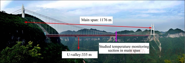
Figure 2 Aizhai suspension bridge

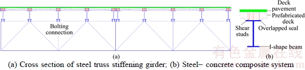
Figure 3 Layout of steel–concrete composite deck system:

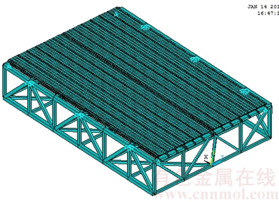
Figure 4 Layout of finite element model

3.2 Full field temperature measurement and results

3.2.1 Full field temperature measurement technique

More than 300 sensors were installed at different locations of the bridge for collecting various types of structural and environmental information. The position of the temperature sensors in the middle of the main span for the Aizhai Suspension Bridge is plotted in Figure 2.

Three groups of temperature sensors were mounted on the section, as shown in Figure 5(a). At each detail, two sensors (W₁ and W₆) measured the temperature of the concrete deck, whereas the other six measured the temperature distribution of the truss trough. The sampling frequency of all the temperature sensors is 1 Hz.

3.2.2 Full field temperature measurement results

Based on the mounted temperature seniors in the health monitoring system, the real-time temperature could be measured and stored. The temperature data within one year were used for the analysis. According to our observations, when the sun was directly over the bridge at noon, the vertical temperature gradient reaches its peak value. The temperature at the same height of the composite structure was almost the same and the temperature gradient across the deck was ignored [6, 7]. Using the calculation model suggested by the current code in China as shown in Figure 5(b) [9], the average value (T₁) for W₁ and W₆ was taken as the real-time temperature on the top of the concrete deck. The average value (T₂) for W₂, W₄, and W₇ was taken as the real-time temperature on the bottom of the concrete deck, whereas the average value (T₃) for W₃, W₅ and W₈ was taken as the real-time temperature on the bottom of the steel truss. Thus, the daily maximum of the vertical temperature gradient could be acquired. Similarly, the monthly maximum of the vertical temperature gradient from January to December in 2013 could be selected, as presented in Figure 6.

In Figure 6, the monthly maximum temperatures for T₁, T₂, and T₃ ranged from 6.7 °C to 54.4 °C, -3.1 °C to 30.1 °C, and -4.4 °C to 31 °C, respectively. The highest vertical temperature gradient appeared in August and the lowest appeared in February. In August, the relative difference was 24.3 °C between T₁ and T₂ and 0.9 °C between T₂ and T₃. The relative difference in February was 9.8 °C between T₁ and T₂ and 1.3 °C for T₂ and T₃. The differences were mainly induced by seasonal temperature fluctuation. The change was consistent with the climate statistics yearbook data of the local meteorological department. In addition, the temperature difference between the top of the I-shaped steel beam (the bottom of concrete deck) and the bottom of steel truss stiffening girder was the minimal throughout the year; the maximum difference ranged from 0.9 °C to 1.3 °C. This trend was caused by the fact that the thermal conductivity of steel is higher than that of concrete. Comparing T₂ and T₃ demonstrated that the difference between the two values was not large. A simplified calculation model of the vertical temperature gradient is proposed, as shown in Figure 5(c). In Figure 5(c), T₄ is taken as the equivalent temperature for steel structural parts; this value is the average of T₂ and T₃. Figure 6 can be simplified as shown in Figure 7 and they are almost identical.

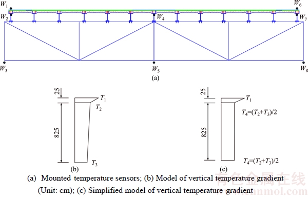
Figure 5 Layout of temperature sensors and calculation model of vertical temperature gradient:

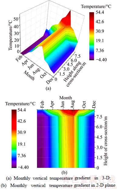
Figure 6 Monthly distribution of maximum vertical temperature gradient:

3.3 FEM-based structural response and stress analysis

Based on the finite element model and the simplified vertical temperature gradient, as shown in Figures 4 and 7, structural analysis is performed to determine the effects of the vertical temperature gradient on the steel–concrete composite structure. The stress and deformation of steel and concrete could be determined for different months. Given the length limitation of this paper, the stress distribution for February and August alone was selected as special case and illustrated in Figure 8.

Figure 8 shows that extreme stress usually happens in the second segment. During subsequent analysis, the second segment was selected for analysis. After the computation, the extreme stress of the vertical temperature gradient in different months for the concrete deck, the I-shaped steel beam, and the steel truss stiffening girder was compared, as shown in Figures 9 to 11. Figure 9 shows that the maximum tensile stress was 4.60 MPa, whereas that of the compressive stress was 6.25 MPa; both values appeared in August. In other months, the range of the extreme stress for tensile change was from 1.67 MPa to 3.46 MPa, whereas that for compressive stress was from 2.98 MPa to 5.21 MPa. Obviously, the extreme value of tensile stress caused by temperature gradient exceeded that suggested by the current code. The high tension would cause cracking of the concrete at the point of connection for steel and concrete if the compressive stress storage of concrete bridge deck under dead load is not induced.

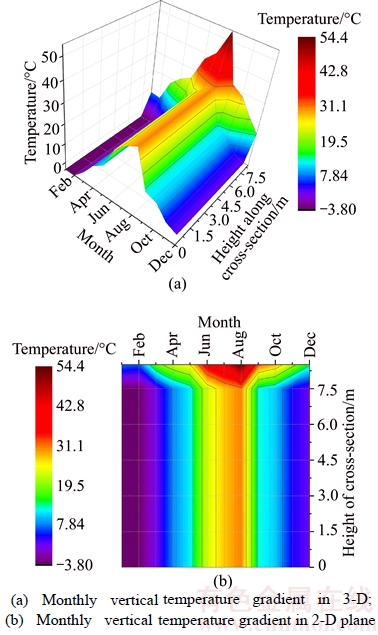
Figure 7 Monthly distribution of simplified maximum vertical temperature gradient:

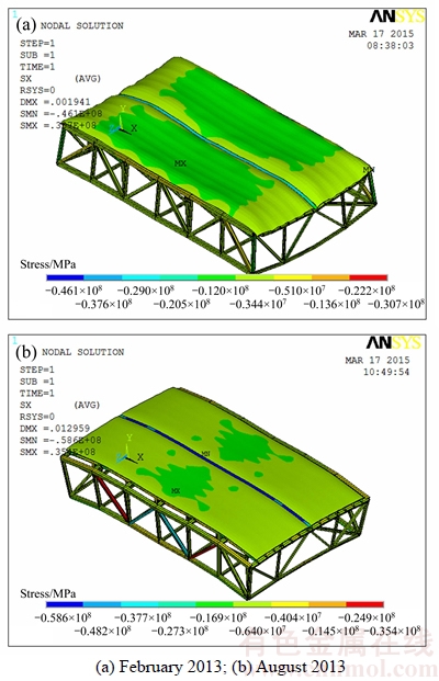
Figure 8 Stress of vertical temperature gradient:

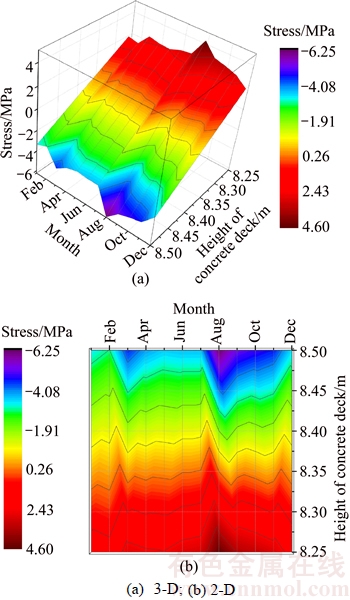
Figure 9 Extreme stress of concrete deck:

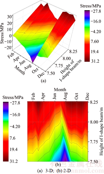
Figure 10 Extreme stress of I-shaped steel beam:

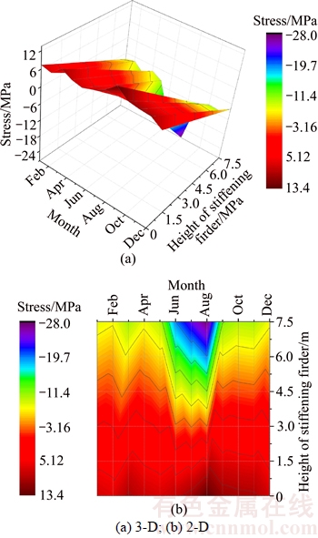
Figure 11 Extreme stress of steel truss stiffening girder:

According to Figure 10, the stress of tension is significantly greater than compressive stress. The largest value of tension was 30.2 MPa, which was found at the position of connection of steel– concrete in August 2013. This difference was mainly induced by the vertical temperature gradient of the concrete deck. Therefore, the variance between T₁ and T₂ was large, whereas that for T₂ and T₃ was small. Consequently, the deformation of the I-shaped steel beam was less than that of the concrete deck. Given the absence of slips on the interface, large tension stress was induced to satisfy the deformation compatibility condition between the concrete and steel on the interface.

In Figure 11, the extreme stress of tension for the steel truss stiffening girder changed within a range of 7.62 MPa to 27.92 MPa, whereas that of compressive stress was 6.62 MPa to 13.4 MPa. Although the stress did not exceed the allowed limit, the largest value of stress was nearly 16.4% of the allowable limit, which requires more attention.

4 Discussions

4.1 Comparison of FEM with existing simplified analysis method

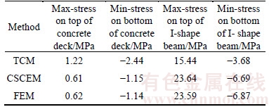
To verify the validity of FEM for calculating the vertical temperature gradient effect, a classic steel–concrete composite structure was used, as shown in the example in Figure 12. The elastic modulus of concrete (E_h) and steel (E_s) are 3.25×10⁴ and 2.10×10⁵MPa, respectively. A comparison of the vertical temperature gradient effect by TCM [9], CSCEM [15], and FEM is presented in Table 1.

Table 1 clearly shows that the difference between the results of TCM and CSCEM or FEM is large, whereas that between CSCEM and FEM is relatively small. The lower level of accuracy for TCM is caused by the shared bending moment for the composite parts of the structure, which are distributed according to distance of the centroid to the composite structure’s neutral axis. Meanwhile, CSCEM and FEM are based on the deformation coordination, the shared bending moments distributed according to the ratio of bending stiffness. The calculation results are close to the real values. Obviously, CSCEM and FEM have higher accuracy for the simple example, while, the former is only suitable for the calculation of the two-dimensional structure [15]. It can be found that TCM and CSCEM suggested by the current code in China are not meeting the accuracy requirements for the calculation of complex 3-D structure. FEM is the best choice for large-scale space composite structures and complex temperature gradients, such as in the calculation of the vertical temperature gradient effect on the steel–concrete composite bridge deck system in suspension bridges.

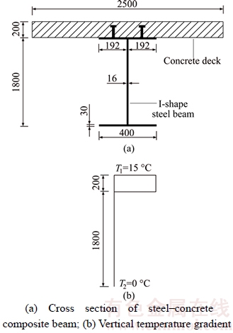
Figure 12 Classic example of steel–concrete structure (Unit: mm):

Table 1 Stress comparison of vertical temperature gradient effect

4.2 Effect of ambient temperature and vertical temperature gradient

The effect of ambient temperature and vertical temperature gradient influences are always mixed together; thus, the analysis becomes rather complex. To determine the relationship of the two factors based on three ambient temperatures and 10 vertical temperature gradients, different cases were established as illustrated in Figure 13.

Figure 13 shows the results for three ambient temperatures (T₄): 6.7°C, 20°C and 26.7°C. For each ambient temperature, 10 temperature gradients (T₁–T₄) ranged from 0°C to 45°C, which were increased by 5°C. In Figure 13(a), T₄ was 6.7°C, and T₁ ranged from 6.7°C to 51.7°C and increased by 5°C. In Figure 13(b), T₄ was 20°C, whereas T₁ ranged from 20°C to 65°C and increased by 5°C. In Figure 13(c), T₄ was 26.7°C, whereas T₁ ranged from 26.7°C to 71.7°C and increased by 5°C.

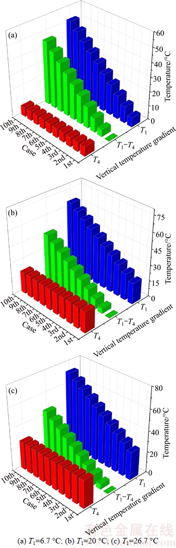
Figure 13 Cases with different ambient temperature:

A combination with the FE model results is shown in Figure 8 and the data are summarized in Figure 13. Thus, effect of ambient temperature and vertical temperature gradient were analyzed. The extreme values of stress for the concrete deck, horizontal I-shaped steel beam, and steel truss stiffening girder were obtained, as shown in Figure 14.

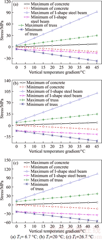
Figure 14 Extreme stress of temperature gradient:

Comparison of Figures 13 and 14 shows that the vertical temperature gradient almost linearly influences the extreme stress of the concrete deck, I-shaped steel beam, and steel truss stiffening girder. Consequently, the function of temperature effects on the temperature gradient is fitted as Eq. (12) by linear regression. Details of the fitting are listed in Table 2.

                            (12)

where σ_ext is the extreme stress; A is the stress coefficient for the temperature gradient; B is the original stress based on the ambient temperature; Δt is the vertical temperature gradient.

Table 2 shows that the value of coefficient A for the max-stress of the concrete deck ranged from 0.168 to 0.170, and that for the min-stress ranged from -0.279 to -0.281. The value of coefficient A for the max-stress of I-shaped steel beam ranged from 1.967 to 1.974, and that for the min-stress ranged from -0.242 to -0.250. The value of coefficient A for the max-stress of the steel truss stiffening girder ranged from 0.577 to 0.604, and that for the min-stress ranged from -0.693 to -0.694. It could be concluded that the variation of coefficient A was not obvious, and the coefficient A was decided by the components of the structure and unaffected by ambient temperature or vertical temperature gradient.

A comparison of Eq. (12), Table 2 against Figure 14 showed that the variation of coefficient B was obvious, and that was decided by the structural components and ambient temperature.

4.3 Effect of vertical temperature gradient calculation model

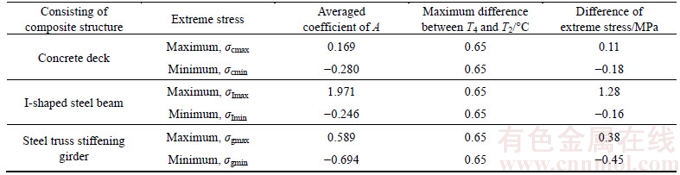
Based on Figures 5(b)–(c) and combined Figures 6 and 7, the biggest difference between T₂ and T₃ was 1.3 °C. After simplification, the biggest difference between T₂ and T₄ was 0.65 °C, which was similar to T₃ and T₄. By considering these differences in Eq. (12) and combining the data with the coefficients illustrated in Table 2, the biggest difference for the extreme values of the concrete deck, I-shaped steel beam, and steel truss stiffening girder could be acquired as illustrated in Table 3.

From Table 3, based on the averaged coefficients of A, the difference in extreme stress was calculated using the difference between T₄ and T₂. The different extreme stress between T₄ and T₂ for the concrete deck was 0.11 and -0.18 MPa, for the I-shaped steel beam was 1.28 and -0.16 MPa, and for the steel truss stiffening girder was 0.38 and -0.45 MPa. Obviously, the different extreme stress induced by the difference between the vertical temperature gradient models shown in Figures 5(b) and (c) was not significant. The simplified model for the vertical temperature gradient has acceptable accuracy.

Table 2 Linear regression of samples

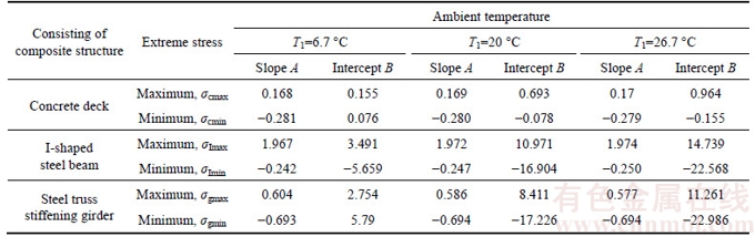
Table 3 Comparison of calculation model

5 Conclusions

1) The proposed FEM can be directly used to realize the thermal calculation of complex structures, without extra assumption and equivalent. The superiority of this method is outstanding compared with other previously mentioned analytical methods.

2) The proposed bilinear model for the temperature gradient in this paper can simplify the complexity of the process and effectively ensure the accuracy of the results of the temperature gradient effect, which is suitable for other similar structures.

3) The largest temperature difference is distributed along the vertical direction of the concrete deck. The height for concrete deck is far smaller than that of the lower steel truss. Thus, the effect of the temperature gradient is concentrated in the region of the former, especially for the interface of concrete and steel. Consequently, stress monitoring should be enhanced in practice.

4) The field results indicated that the temperature gradient and its effects are larger than what is suggested in the current codes. Therefore, in subsequent applications, the factor of safety should be approximately improved according to the characteristics of the structure.

5) In the aforementioned steel–concrete deck system, the linearity relations between the stress and temperature gradient are outstanding. The extreme value of stress can be rapidly acquired with the linear expressions, which are convenient and can be widely popularized during the elevation of temperature gradient effects.

References

[1] DING Y L, LI A Q, GENG F F. Damage warning of suspension bridges based on neural networks under changing temperature conditions [J]. Journal of Southeast University: Eng Edi, 2010, 26(4): 586–590. (in Chinese)

[2] CHOI C K, NOH H C. Ultimate strength of RC cooling tower shells subjected to temperature and wind loads [J]. J Korean Soc Civ Eng, 1999, 19(14): 469–469.

[3] SALAWU O S. Detection of structural damage through changes in frequency: A review [J]. Eng Struct, 1997, 19(9): 718–723.

[4] GIUSSANI F. The effects of temperature variations on the long-term behavior of composite steel-concrete beams [J]. Eng Struct, 2009, 31(10): 2392–2406.

[5] CHEN X Q, LIU Q W, ZHU J. Measurement and theoretical analysis of solar temperature field in steel-concrete composite girder [J]. Journal of Southeast University: Eng Edi, 2009, 25(4): 513–517. (in Chinese)

[6] XIA Y, CHEN B, ZHOU X Q, XU Y L. Field monitoring and numerical analysis of Tsing Ma Suspension Bridge temperature behavior [J]. Struct Control Health Monit, 2013, 20(4): 560–575.

[7] DING Y L, WANG G X, ZHOU G D. Life-cycle simulation method of temperature field of steel box girder for Runyang cable-stayed bridge based on field monitoring data [J]. China Civ Eng, 2013, 46(5): 129–136. (in Chinese)

[8] EUROCODE C E N. Design of composite steel and concrete structures II: Bridges [S]. European Committee for Standardization, 1994.

[9] JTG D62–2004. Design code for design of highway reinforced concrete and pre-stressed concrete bridge culvert [S]. China, 2004. (in Chinese)

[10] AASHTO. AASHTO LRFD bridge design specifications [S]. Washington D.C: AASHTO, 2007.

[11] KOCATURK T, AKBAS S D. Thermal post-buckling analysis of functionally graded beams with temperature- dependent physical properties [J]. Steel Comp Struct, 2013, 15(5): 481–505.

[12] O, HAKTANIR T, ALTUN F. Experimental research for the effect of high temperature on the mechanical properties of steel fiber-reinforced concrete [J]. Constr Build Mater, 2015, 75: 82–88.

[13] XIA Y, HAO H, ZANARDO G, DEEKS A. Long term vibration monitoring of an RC slab: temperature and humidity effect [J]. Eng Struct, 2006, 28(3): 441–452.

[14] MACDONALD J H, DANIELL W E. Variation of modal parameters of a cable-stayed bridge identified from ambient vibration measurements and FE modeling [J]. Eng Struc, 2005, 27(13): 1916–1930.

[15] YIN C X. Computing method for effect analysis of temperature and shrinkage on steel-concrete composite beams [J]. China J Hwy Trans, 2014, 27(11): 76–83. (in Chinese)

[16] ZIVICA V, KRAJCI L, BAGEL L, VARGOVA M. Significance of the ambient temperature and the steel material in the process of concrete reinforcement corrosion [J]. Constr Build Mater, 1997, 11(2): 99–103.

[17] THURSTON S J, PRIESTLEY M J N, CDOKE N. Thermal analysis of thick concrete sections [J]. ACI J, 1980, 77(5): 347–357.

[18] ELBADRY M M, GHALI A. Temperature variation in concrete bridges [J]. Journal of Structural Engineering, 1983, 109(10): 2355–2374.

[19] DENG J, LEE M M K, LI S. Flexural strength of steel–concrete composite beams reinforced with a prestressed CFRP plate [J]. Constr Build Mater, 2011, 25(1): 379–384.

[20] XU X, LIU Y, HE J. Study on mechanical behavior of rubber-sleeved studs for steel and concrete composite structures [J]. Constr Build Mater, 2014, 53: 533–546.

[21] ATTIA A, TOUNSI A, BEDIA E A, MAHMOUD S R. Free vibration analysis of functionally graded plates with temperature-dependent properties using various four variable refined plate theories [J]. Steel Comp Struct, 2015, 18(1): 187–212.

[22] RIDING K A, POOLE J L, SCHINDLER A K, JUENGER M C, FOLLIARD K J. Temperature boundary condition models for concrete bridge members [J]. ACI Mater J, 2007, 104(4): 379–387.

(Edited by YANG Hua)

中文导读

悬索桥钢–混组合桥面系温度梯度数值模拟及效应研究

摘要：对钢–混组合结构温度梯度效应的研究，主要是以竖向温度梯度结合二维有限元模型开展的；而对大跨度桥梁实测温度梯度的研究发现，其具有典型的空间特性。鉴于此，以矮寨大桥为研究背景，对大跨度悬索桥钢–混组合桥面系的周年实测空间温度梯度进行实测研究，建立大跨度悬索桥钢–混组合桥面系的空间有限元节段模型，研究在空间温度梯度耦合作用下，桥面系结构参数与力学响应之间的关系，得出的结论可为同类结构的建养提供有益的参考。

关键词：悬索桥；钢–混组合桥面系；竖向温度梯度；有限元法；温度应力

Foundation item: Project(2015CB057701) supported by the National Basic Research Program of China; Project(51308071) supported by the National Natural Science Foundation of China; Project(13JJ4057) supported by Natural Science Foundation of Hunan Province, China; Project(201408430155) supported by the Foundation of China Scholarship Council; Project(2015319825120) supported by the Traffic Department of Applied Basic Research, China; Project(12K076) supported by the Open Foundation of Innovation Platform in Hunan Provincial Universities, China

Received date: 2017-04-20; Accepted date: 2017-12-10

Corresponding author: DENG Yang, Associate Professor, PhD; E-mail: seudengyang@foxmail.com; ORCID: 0000-0001-5807-1440