J. Cent. South Univ. (2012) 19: 1892-1901 

DOI: 10.1007/s11771-012-1223-y

Data-driven nonlinear control of a solid oxide fuel cell system

LI Yi-guo(李益国)¹, SHEN Jiong(沈炯)¹, K. Y. Lee ², LIU Xi-chui(刘西陲)¹, FEI Wen-zhe(费文哲)¹

1. Key Laboratory of Energy Thermal Conversion and Control of Ministry of Education

(School of Energy and Environment, Southeast University), Nanjing 210096, China;

2. Department of Electrical and Computer Engineering, Baylor University, Waco, TX 76798-7356, USA

? Central South University Press and Springer-Verlag Berlin Heidelberg 2012

Abstract: Solid oxide fuel cells (SOFCs) are considered to be one of the most important clean, distributed resources. However, SOFCs present a challenging control problem owing to their slow dynamics, nonlinearity and tight operating constraints. A novel data-driven nonlinear control strategy was proposed to solve the SOFC control problem by combining a virtual reference feedback tuning (VRFT) method and support vector machine. In order to fulfill the requirement for fuel utilization and control constraints, a dynamic constraints unit and an anti-windup scheme were adopted. In addition, a feedforward loop was designed to deal with the current disturbance. Detailed simulations demonstrate that the fast response of fuel flow for the current demand disturbance and zero steady error of the output voltage are both achieved. Meanwhile, fuel utilization is kept almost within the safe region.

Key words: solid oxide fuel cell (SOFC); data-driven method; virtual reference feedback tuning (VRFT); support vector machine (SVM); anti-windup

1 Introduction

Fuel cells are considered to be one of the most important clean, distributed resources due to their high efficiency and low environmental pollution. Among the various types of fuel cell, the solid oxide fuel cell (SOFC) has attracted considerable interest as it offers a wide range of applications, flexibility in the choice of fuel, high system efficiency etc, but it presents a challenging control problem owing to slow dynamics, nonlinearity and tight operating constraints of the SOFC [1].

Almost all the researches that have been conducted in SOFC control are model-based [2-5], since an explicit model of the SOFC system is required to design controllers. In Ref. [2], a novel offset-free input-to-state stable fuzzy predictive controller was developed, based on the identified fuzzy model. A Hammerstein model, consisting of a radial basis function (RBF) neural network in cascade with an autoregressive exogenous input (ARX) model [3], was adopted to describe the nonlinear dynamic properties of the SOFC. In Ref. [4], a nonlinear model predictive control (MPC) was proposed to control the voltage based on an improved RBF network optimized with genetic algorithm (GA). A MPC based on a fuzzy Hammerstein model for an SOFC was presented in Ref. [5].

Recently, a data-driven linear MPC using subspace system identification [6] was first used to deal with an SOFC system without full online measurement of all output variables. However, because the SOFC system is an uncertain nonlinear system and its structure and parameters vary with the change of operating points, a new data-driven nonlinear controller is required to cope with the nonlinearity of the SOFC system more effectively.

The virtual reference feedback tuning (VRFT) method gives a solution to the problem of designing a controller for a system whose I/O behavior is unknown, on the basis of a single set of I/O data, without resorting to the identification of a model of the system [7-11]. VRFT was originally proposed for linear systems by GUARDABASSI and SAVARESI [7] and developed in Refs. [8-9] in two respects: the design of a pre-filter for the data and the treatment of non-minimum phase plants. In 2007, SALA [10] integrated VRFT into a unified closed-loop identification framework. The VRFT method has also been used to design the adaptive PID controller [11]. However, most of these reports are limited to linear systems.

In this work, a novel data-driven nonlinear control strategy is proposed to solve the SOFC control problem by combining the VRFT method and support vector machine (SVM) technique. In order to fulfill the requirements for fuel utilization and control constraints, a dynamic constraints unit and an anti-windup scheme are adopted. In addition, a feedforward loop is designed to deal with the current disturbance.

2 SOFC system description

The SOFC system includes a fuel processing unit or the reformer and a fuel cell stack. Hydrogen is the main fuel for most types of fuel cell. Nevertheless, other fuels such as methane, methanol, ethanol, gasoline and oil derivatives can also be used when a reformer is included in a fuel cell system for converting the fuel to hydrogen.

The basic components of the SOFC are the anode, cathode and two ceramic electrodes. In the fuel cell, fuel is supplied to the anode and air is supplied to the cathode. At the cathode/electrolyte interface, oxygen molecules accept electrons coming from the external circuit to form oxide ions. The electrolyte layer allows only oxide ions to pass through it and, at the anode/electrolyte interface, hydrogen molecules present in the fuel react with oxide ions to form steam and electrons are released. These electrons pass through the external circuit to reach the cathode/electrolyte layer, and thus the circuit is closed.

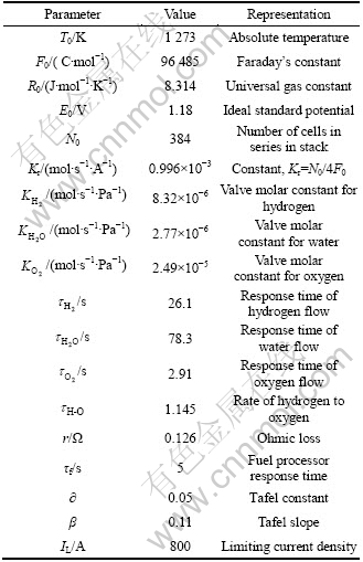
In this work, a widely accepted dynamic model of an SOFC system is adopted [2-6], as shown in Fig. 1, where V_dc denotes the stack output voltage (V), I the external current load (A) and q_f the natural gas flow rate (mol/s). Table 1 contains the parameters of the SOFC model [2].

Applying Nernst’s equation and taking into account ohmic, concentration, and activation losses, the stack output voltage is represented as follows:

                   (1)

      (2)

where

                (3)

                (4)

                        (5)

                                  (6)

                              (7)

                       (8)

3 Considerations for controller design of an SOFC system

The following aspects should be considered in the controller design for the SOFC system:

1) A nonlinear controller is preferred over a linear controller because of the nonlinearity of the SOFC with the change of operating points. The stationary voltage/current characteristics of an SOFC system show that the SOFC exhibits nonlinear behavior over a wide operating regime. The stack voltage usually shows significant changes, especially at low and high current loads, and an overloaded current leads to a rapid deterioration of operating stack voltage.

2) As a measurable disturbance, the current load I should be utilized to construct a feedforward loop to keep the output voltage steady by speeding up the initial response of fuel flow for drastic current changes.

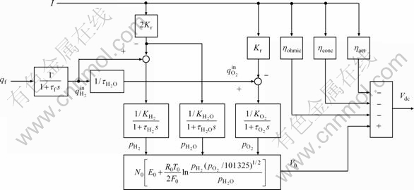
Fig. 1 SOFC system dynamic model

Table 1 Parameters in SOFC system

3) Besides ordinary actuator constraints on the control signal, the fuel utilization of the SOFC system should also be kept within a safe range as long as possible. Fuel utilization is one of the most important operating variables that can affect the performance of an SOFC. Fuel utilization is defined as

                  (9)

where ,  and  are the hydrogen input, output, and reacted flow rates. The desired range of fuel utilization is from 0.7 to 0.9, in order to prevent overused and underused fuel conditions. An overused-fuel condition can lead to permanent damage to the cells due to fuel starvation and an underused-fuel situation results in low efficiency for the SOFC [2-6].

4 Virtual reference feedback tuning and support vector machine

4.1 Virtual reference feedback tuning

VRFT is essentially the model reference control problem shown in Fig. 2, where C(z) is a feedback controller and M(z) is the reference model.

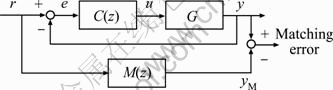
Fig. 2 Model reference control

For standard model reference design methods, a reference model is first selected, and then the controller C(z) is regulated such that the output error between the actual plant and the reference model is minimized. This can be described by

      (10)

where W(z) is a weighting function chosen by the user. However, when the plant is unknown, an indirect method has to be employed, which means that a model must first be identified.

In contrast, the VRFT first constructs a virtual reference  according to the measured y(k) such that Such a reference is called “virtual” because it is not used to generate y(k). However, y(k) can be seen as the desired output of the closed-loop system when the reference signal is . We also know that when the plant G(z) is fed by u(k), it generates y(k) as output. Therefore, a good controller is one that generates u(k) when fed by . Since both signals e(k) and u(k) are known, problem Eq. (10) is thus transformed into the need to minimize Eq. (11), which is an identification problem. The aim of the VRFT approach is not the design of the “best” possible controller, but the design of a controller with good tracking and robustness properties, based on a reduced set of data. So it is tunable in a very short time as follows:

         (11)

where L(z) is a user-chosen filter, and m denotes the number of the measured I/O data.

4.2 Support vector machine

The ε–SVM algorithm [12-13] is briefly reviewed.

Consider the training data set  where x_i is the i-th input data in the input space Rⁿ and y_i∈R is the corresponding output value. The SVM approximates the relationship between the input and output data points in the following form:

                        (12)

where w is a vector in the feature space , f(x_i) is a mapping of the input space to the feature space F, b is the bias term, and á·,·? stands for the inner product   in F.

The ε-SVM model is aimed at minimizing the regularized loss function  based on the following ε-insensitive model:

           (13)

The optimization problem can be formulated as

(14)

where ε is the maximum value of the tolerable error, ξ_i⁺ and ξ_i^- are slack variables, ||·|| is the Euclidean norm, and C is a regularization parameter that represents a trade-off between the model complexity and the tolerance to an error larger than ε. The dual form of Eq. (14) becomes a quadratic programming (QP) problem as follows:

               (15)

where K(x_i, x_j)=, is a kernel function. Motivated by Mercer’s condition, the kernel function handles the inner product in the feature space. Hence, the explicit form of  does not need to be known.

The solution of the QP problem Eq. (15) gives the optimum values of α_i⁺ and α_i^-. Then, one obtains

, where some of the coefficients

(α_i⁺-α_i^-) have non-zero values and the corresponding training data points have an approximation error equal to or greater than ε. When only the support vectors corresponding to non-zero values of β_i=(α_i⁺-α_i^-) are considered, Eq. (12) becomes

                   (16)

where l denotes the number of support vectors in the model. The bias b is calculated as

       (17)

where x_r and x_s are support vectors.

5 Data-driven nonlinear controller design method

5.1 Relation between virtual reference feedback tuning and internal model control

As we know, internal model control (IMC) can be depicted in Fig. 3(a) when the feedforward filter and feedback filter are set to be equal, and F denotes the filter, C′ is an internal model controller and G^* is a model of the plant.

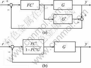
Fig. 3 Internal model control: (a) General IMC structure; (b) Equivalent structure of IMC

Obviously, when there is no mismatch between G and G^*(G=G^*), and the set C′=G^*-1 (and assuming G can be inverted), IMC is an ideal implementation of the minimizing of Eq. (10). In this case, the filter F is equal to the reference model M. Figure 3(a) can be transformed into Fig. 3(b), therefore an ideal controller C⁰ is given by Eq. (18) according to Fig. 3(b). Actually, the aim of VRFT is to approximate to the ideal controller as closely as possible by minimizing Eq. (11).

      (18)

Because VRFT provides closed-loop feedback control, it has the advantage of dealing with disturbance and uncertainty more effectively than direct inverse control, which directly identifies the inverse model of the plant and uses it as a controller. VRFT is also different from IMC which needs to acquire a model of the plant first.

5.2 Nonlinear controller design based on virtual references and support vector machine

5.2.1 Structure of control system

In VRFT, the controller design problem is transformed into an identification problem. This work employs SVM to solve this problem and therefore gives a specific implementation of nonlinear VRFT. SVM is chosen because of the following properties: 1) It is good at generalization and approximating nonlinearity, especially when the training samples are limited; 2) Its solution is unique after the samples are fixed. This is due to the fact that support vector regression is formulated as a convex quadratic optimization problem which has a global optimum. Hence, the design results can be repeated; 3) SVM can cope with noise effectively because of the application of an ε-insensitive function; 4) It is convenient to change the design results by tuning the SVM parameters. These properties determine that SVM is more suitable than a neural network as a controller in this problem.

In real applications, a reference model is often set up in the form of a transfer function:

             (19)

As a result, the ideal controller C⁰ can be expressed by

      (20)

According to Eq. (20), the ideal controller C⁰ consists of the integral action. Therefore, a discrete control system is constructed, as shown in Fig. 4, in which the integral action is extracted artificially, and SVM is employed to approximate the rest of C⁰. Due to the above treatment, the following advantages can be achieved: 1) The steady-state error can be eliminated; 2) The complexity is reduced by identifying a stable object instead of an unstable one. Actually, this controller can be regarded as a nonlinear integral controller with variable gain.

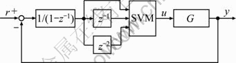
Fig. 4 Nonlinear controller based on virtual references and support vector machine

5.2.2 Procedure for design of controller

Step 1: Acquire a set of measured I/O data  from an unknown plant. The samples should reach the possible operating regime;

Step 2: Get the new data set  by pre-filtering the measured I/O data  with a suitable filter L(z);

Step 3: Select a reference model M(z)=M′(z)z^-(d+1)= , where d denotes the delay time, which means that the reference model has at least one step delay;

Step 4: Calculate the corresponding virtual reference , which means that the virtual reference in step i should be constructed at least in terms of the output in step i+1 (when d=0);

Step 5: Calculate the error then compute S_i=S_i-1+e_i;

Step 6: Organize training samples of SVM using x_i=[S_i-2 S_i-1 S_i]^T as input variables and  as output variables, where i=1, 2, …, m₁ (m₁=m-d-1);

Step 7: Set the parameters of the SVM, including weighting coefficient C, the width parameter σ (in which the Gaussian kernel function is adopted) and ε.

The simulation results demonstrate that σ has more effect on the design results than C. Too small C will result in insufficient learning from the training data, while too large C leads to overfitting. σ and C affect the generalization ability of the SVM in opposite directions. Increasing the values of ε and σ properly can give the controller greater ability for dealing with noise [14], which can be observed from the simulations.

Step 8: Construct and solve the optimization problem Eq. (14).

The optimization problem Eq. (14) is effectively solved by its dual problem Eq. (15) using the sequential minimal optimization (SMO) algorithm [15]. The values of α_i⁺ and α_i^- are determined and the designed nonlinear controller can be expressed as

             (21)

6 Data-driven nonlinear control of SOFC system

6.1 Structure of data-driven nonlinear control system for SOFC

Based on the approach proposed above, the specific data-driven nonlinear control system is designed for an SOFC system, as shown in Fig. 5. It is a compound control system consisting of both feedforward and feedback loops. As a measurable disturbance, the current density I is introduced as part of the input variables of the SVM in the nonlinear controller to speed up the initial response of fuel flow to drastic current changes. The feedback loop with an integrator ensures an offset free of the output voltage in the case of load step changes. A dynamic constraint unit and an anti-windup scheme are also adopted to guarantee fuel utilization within the desired region. The SVM model in the nonlinear controller is identified according to Fig. 6 using a SMO algorithm. x_k=[I_k-2 I_k-1 I_k S_k-2 S_k-1 S_k]^T is chosen as its input.

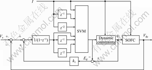
Fig. 5 Structure of data-driven nonlinear control of SOFC system

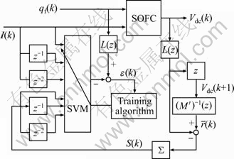
Fig. 6 Identification structure of nonlinear controller of SOFC system

6.2 Dynamic constraints and anti-windup scheme

Assuming that the safe range of fuel utilization is within [u_f,min, u_f,max], and the actuator constraints on control signal are [q_f,min, q_f,max], the dynamic constraints unit in Fig. 5 is designed as follows.

In terms of Eq. (9), to guarantee safe utilization, the hydrogen flow should be within , where =2K_rI(k)/u_f,max and = 2K_rI(k)/u_f,min.

Because it is appropriate to approximate the fuel processing unit using a first-order transfer function, we can calculate the constraints  on the fuel flow (the natural gas flow rate) backwards from . For example, in the case of sample time T_s=1 s,  0.181 3,  So, the final dynamic constraints  on the fuel flow can be calculated using

                     (22)

                     (23)

The introduction of the integrator may suffer from integrator windup, in which the feedback loop becomes temporarily disconnected since the controller output is no longer affected by the feedback signal. So, an anti-windup scheme is used to reduce integrator windup in Fig. 5 by feeding back the error signal E_d, which is the difference between the required control signal and the actual control signal.

7 Simulations

The proposed data-driven nonlinear controller discussed above is applied to the SOFC problem to achieve safe fuel utilization and maintain operating constraints when only the voltage output is measurable online. The sampling rate of the SOFC and the nonlinear controller is chosen as T_s=1 s.

7.1 Design of data-driven nonlinear controller

The open-loop input–output data are required to design the data-driven nonlinear controller. Open loop input–output data samples are obtained by exciting the open loop SOFC system using designed sine signals 0.782 3+0.3sin(0.5t)sint and 300+50sin(0.03t)sin(0.04t) for the fuel and the current demand, respectively, which are collected over 1 000 s. All the 1 000 sampled data points are divided into two sets: the training set and testing set, where the training set contains 900 data points and the testing set contains the remaining 100 data points. The reference model is selected as

and the filter is set to be L(z)=1.

First, the SVM in the nonlinear controller is identified in term of Fig. 6 with different parameter settings, giving the results shown in Table 2. The quality of approximation is measured using the root mean square error (RMSE) between the samples and the SVM:

               (24)

Table 2 Training and test results with different parameter settings

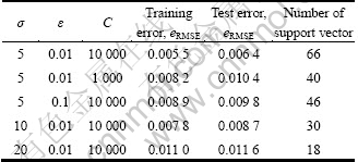
In order to make a trade-off between the accuracy and the complexity of the nonlinear controller, we choose C=10 000, ε=0.01, σ=10 in terms of the testing error and the number of support vectors in the following simulations. The corresponding training and test results are plotted in Fig. 7, which show that the SVM can approximate the behavior of the nonlinear controller with good accuracy.

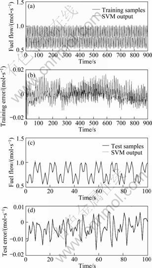
Fig. 7 Training ((a) and (b)) and test ((c) and (d)) results of nonlinear controller: (a) and (c) Fuel flow; (b) and (d) Test error

7.2 Data-driven nonlinear control of SOFC system

As an independent power source candidate, the output voltage of the SOFC system is expected to be at a desired constant value for stable operation of external electrical equipment. The external load will directly affect the output voltage of the SOFC system.

In normal working conditions, the current of the SOFC system is 300 A. The steady output of the voltage is 333 V. Assuming that a load disturbance causes multiple step changes of the current, which decreases from 300 A to 280 A when t=50 s, changes from 280 A to 320 A when t=200 s and goes back to 290 A after t=350 s, the data-driven nonlinear controller is used to adjust the voltage to its steady value. For all simulations, the following parameters are set: anti-windup feedback coefficient k₁=5, [q_f,min, q_f,max]=[0, 1.2] mol/s, [u_f,min, u_f,max]=[0.7, 0.9].

By applying the proposed nonlinear controller, satisfactory control performances are achieved for the closed-loop SOFC system for large current load step changes, as shown in Fig. 8. It is observed from Fig. 8 that the fast response of fuel flow for the current demand disturbance and zero steady error of the output voltage are both achieved. Meanwhile, fuel utilization is kept almost within the safe region except for a brief deviation at t=200 s. Note that the fuel utilization cannot be definitely restricted to the desired range for large and sudden current load changes because of the slow response of the fuel flow to the output voltage and constraints on the fuel flow.

To demonstrate the effects of the feedforward loop and the dynamic constraints, simulations in two other cases were performed.

Case 1: Without feedforward loop

Simulations were carried out under the same conditions as those in Fig. 8 except that the current feedforward input to the nonlinear controller was kept at 300 A, with the results shown in Fig. 9. By comparing Fig. 9 with Fig. 8, it is clear that the initial response of fuel flow became slow, which resulted in a larger and longer dynamic error of the output voltage.

Case 2: Without dynamic constraints unit

Simulations were performed using the same conditions as those in Fig. 8 except that the dynamic constraints unit was replaced with the normal maximum and minimum constraints on control input signal, giving the results shown in Fig. 10. By comparing Fig. 10 with Fig. 8, it is clear that the fuel utilization can no longer be kept within the desired safe range for the current disturbances at t=50 s and t=350 s without the dynamic constraints unit.

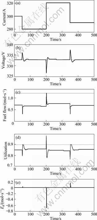
Fig. 8 Simulation results of proposed nonlinear controller under current step disturbance: (a) Current; (b) Voltage; (c) Fuel flow; (d) Utilization; (e) E_d

The effect of the anti-windup scheme can also be observed from Fig. 8(e) and Fig. 10(e).

7.3 Dealing with noisy data

Because the samples are always affected by noise, the ability of proposed approach in dealing with noisy data is checked. We assume that the output voltage of the SOFC is affected by additive colored noise C(z^-1)ξ(k), where C(z^-1)=1-0.3574z^-1-0.033 92z^-2 and ξ(k) is white noise with power of 0.3. In order to reduce the influence of noise, a filter L(z)=0.632 1/(z-0.367 9) was applied.

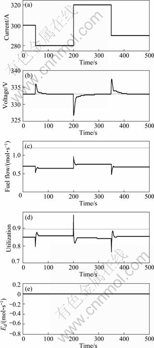
Fig. 9 Simulation results without feedforward loop: (a) Current; (b) Voltage; (c) Fuel flow; (d) Utilization; (e) E_d

To make the nonlinear controller more robust to noise, we change the parameters in training the SVM model, giving the training and test results in Table 3. Notice that the identification accuracy is degraded with respect to the noise-free case.

For this very noisy condition, satisfactory closed-loop response can be achieved by applying the nonlinear controller, as shown in Fig. 11, demonstrating that the proposed approach can deal effectively with noisy data by setting the relevant parameters properly. The instrumental variable method can be used to further counteract the effect of noise [8], by repeated experiment or the identification of the plant.

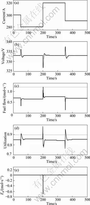
Fig. 10 Simulation results without dynamic constraints: (a) Current; (b) Voltage; (c) Fuel flow; (d) Utilization; (e) E_d

Table 3 Training and test results of nonlinear controller on noisy data

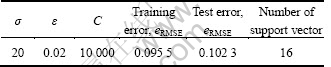
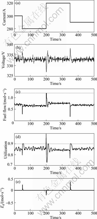
Fig. 11 Closed-loop response for noisy condition: (a) Current; (b) Voltage; (c) Fuel flow; (d) Utilization; (e) E_d

8 Conclusions

1) A data-driven nonlinear control strategy has been developed by combining a virtual reference feedback tuning method and support vector machine for the SOFC system, which provides an alternative to the SOFC control problem. A feedforward loop is designed to speed up the initial response of fuel flow and a dynamic constraints unit with anti-windup scheme is adopted to keep fuel utilization within a safe range as long as possible and eliminate integrator windup.

2) This approach is particularly effective for SOFC since the explicit dynamic model of SOFCs is generally difficult to develop.

3) The simulation results have validated the proposed data-driven nonlinear control algorithm. Dealing with noisy data is also verified by simulations. One future research topic is to introduce the instrumental variable method to further counteract the effect of noise.

References

[1] Knyazkin V, Soder L, Canizares C. Control challenges of fuel cell-driven distributed generation [C]// IEEE Power Tech Conference. New York: IEEE, 2003: 328-333.

[2] Zhang Tie-jun, Feng Gang. Rapid load following of a SOFC power system via stable fuzzy predictive controller [J]. IEEE Trans on Fuzzy Systems, 2009, 17(2): 357-371.

[3] Huo Hai-bo, Zhong Zhi-dan, Zhu Xin-jian, Tu Heng-yong. Nonlinear dynamic modeling for a SOFC stack by using a Hammerstein model [J]. Journal of Power Sources, 2008, 175(1): 441-446.

[4] Wu Xiao-juan, Zhu Xin-jian, CAO Guang-yi, TU Heng-yong. Predictive control of SOFC based on a GA-RBF neural network model [J]. Journal of Power Sources, 2008, 179(1): 232-239.

[5] Jurado F. Predictive control of solid oxide fuel cells using fuzzy Hammerstein models [J]. Journal of Power Sources, 2006, 158(1): 245-253.

[6] Wang Xiao-rui, Huang Biao, Chen Tong-wen. Data-driven predictive control for solid oxide fuel cells [J]. Journal of Process Control, 2007, 17(2): 103-114.

[7] Guardabassi G O, Savaresi S M. Virtual reference direct design method: An off-line approach to data-based control system design [J]. IEEE Trans on Automatic Control, 2000, 45(5): 954-959.

[8] Campi M C, Lecchini A, Savaresi S M. Virtual reference feedback tuning: A direct method for the design of feedback controllers [J]. Automatica, 2002, 38(8): 1337-1346.

[9] CAMPESTRINI L, ECKHARD D, GEVERS M, BAZANELLA A S. Virtual reference feedback tuning for non-minimum phase plants [J]. Automatica, 2011, 47(8): 1778-1784.

[10] Sala A. Integrating virtual reference feedback tuning into a unified closed-loop identification framework [J]. Automatica, 2007, 43(1): 178-183.

[11] KANSHA Y, HASHIMOTO Y, CHIU M. New results on VRFT design of PID controller [J]. Chemical Engineering Research and Design, 2008, 86(8): 925-931.

[12] Scholkopf B, Smola A J. Learning with kernels: Support vector machines, regularization, optimization and beyond [M]. Cambridge, MA: MIT Press, 2002: 251-271.

[13] NIU Dong-xiao, WANG Yong-li, MA Xiao-yong. Optimization of support vector machine power load forecasting model based on data mining and Lyapunov exponents [J]. Journal of Central South University of Technology, 2010, 17(2): 406-412.

[14] Cherkassky V, Ma Y. Practical selection of SVM parameters and noise estimation for SVM regression [J]. Neural Networks, 2004, 17(1): 113-126.

[15] Flake G W, Lawrence S. Efficient SVM regression training with SMO [J]. Machine Learning, 2002, 46(1/2/3): 271-290.

(Edited by YANG Bing)

Foundation item: Projects(51076027, 51036002) supported by the National Natural Science Foundation of China; Project(20090092110051) supported by the Doctoral Fund of Ministry of Education of China

Received date: 2011-04-13; Accepted date: 2011-07-22

Corresponding author: LI Yi-guo, Associate Professor, PhD; Tel: +86-25-83795951-804; E-mail: lyg@seu.edu.cn