A novel Lagrangian relaxation level approach for scheduling steelmaking-refining-continuous casting production
��Դ�ڿ������ϴ�ѧѧ��(Ӣ�İ�)2017���2��
�������ߣ����¸� ���� ��ȫ�� ������ ��ʤƽ
����ҳ�룺467 - 477
Key words��steelmaking-refining-continuous casting; Lagrangian relaxation (LR); approximate subgradient optimization
Abstract: A Lagrangian relaxation (LR) approach was presented which is with machine capacity relaxation and operation precedence relaxation for solving a flexible job shop (FJS) scheduling problem from the steelmaking-refining-continuous casting process. Unlike the full optimization of LR problems in traditional LR approaches, the machine capacity relaxation is optimized asymptotically, while the precedence relaxation is optimized approximately due to the NP-hard nature of its LR problem. Because the standard subgradient algorithm (SSA) cannot solve the Lagrangian dual (LD) problem within the partial optimization of LR problem, an effective deflected-conditional approximate subgradient level algorithm (DCASLA) was developed, named as Lagrangian relaxation level approach. The efficiency of the DCASLA is enhanced by a deflected-conditional epsilon-subgradient to weaken the possible zigzagging phenomena. Computational results and comparisons show that the proposed methods improve significantly the efficiency of the LR approach and the DCASLA adopting capacity relaxation strategy performs best among eight methods in terms of solution quality and running time.
Cite this article as: PANG Xin-fu, GAO Liang, PAN Quan-ke, TIAN Wei-hua, YU Sheng-ping. A novel Lagrangian relaxation level approach for scheduling steelmaking-refining-continuous casting production [J]. Journal of Central South University, 2017, 24(2): 467-477. DOI: 10.1007/s11171-017-3449-9.
J. Cent. South Univ. (2017) 24: 467-477
DOI: 10.1007/s11171-017-3449-9

PANG Xin-fu(���¸�)1, 2, GAO Liang(����)1, PAN Quan-ke(��ȫ��)1,
TIAN Wei-hua(������)2, YU Sheng-ping(��ʤƽ)3
1. State Key Laboratory of Digital Manufacturing Equipment and Technology (Huazhong University of
Science and Technology), Wuhan 430074, China;
2. School of Automation, Shenyang Institute of Engineering, Shenyang 110136, China;
3. State Key Laboratory of Synthetical Automation for Process Industries (Northeastern University),Shenyang 110819, China
 Central South University Press and Springer-Verlag Berlin Heidelberg 2017
Abstract: A Lagrangian relaxation (LR) approach was presented which is with machine capacity relaxation and operation precedence relaxation for solving a flexible job shop (FJS) scheduling problem from the steelmaking-refining-continuous casting process. Unlike the full optimization of LR problems in traditional LR approaches, the machine capacity relaxation is optimized asymptotically, while the precedence relaxation is optimized approximately due to the NP-hard nature of its LR problem. Because the standard subgradient algorithm (SSA) cannot solve the Lagrangian dual (LD) problem within the partial optimization of LR problem, an effective deflected-conditional approximate subgradient level algorithm (DCASLA) was developed, named as Lagrangian relaxation level approach. The efficiency of the DCASLA is enhanced by a deflected-conditional epsilon-subgradient to weaken the possible zigzagging phenomena. Computational results and comparisons show that the proposed methods improve significantly the efficiency of the LR approach and the DCASLA adopting capacity relaxation strategy performs best among eight methods in terms of solution quality and running time.
Key words: steelmaking-refining-continuous casting; Lagrangian relaxation (LR); approximate subgradient optimization
1 Introduction
As one of major bottlenecks in the iron and steel production, steelmaking-refining-continuous casting (SCC) process including steelmaking, refining and continuous casting, is a complicated flexible manufacturing process, which needs expensive and energy-intensive equipments running in continuous mode. Therefore, an effective and efficient SCC scheduling is crucial to improve productivity of the entire production system and save manufacturing cost [1]. The SCC scheduling problems can be broadly classified into two groups: hybrid flow shop (HFS) and flexible job shop (FJS). The main difference between the two groups is in the refining stage, where there are multiple process steps, e.g., Rushrstal Heraeus (RH) process, Ladle Furnace (LF) process, and Injection Refining-up Temperature (IR_UT) process. In the FJS, the jobs undergo different routes. Some jobs are refined from RH to LF, whereas the others are from RH to IR_UT or from LF to IR_UT (seen in Section 2.1). In the literature, most of the studies on SCC scheduling problem focused on the HFS-type [2-12]. This work addresses the FJS-type scheduling problem that has received little attention in the literature but can be commonly found in real-world SCC process.
Although exact algorithms such as branch-and-cut algorithm and the algorithm based on the disjunctive graph have been developed, they are only applicable to small-scale FJS problems because of their NP-hard natures. Therefore, heuristic approach [13] is proposed to get high quality solutions within an acceptable computational time. LR approach is also a near optimal method, which can not only generate a near-optimal schedule in a reasonable computational time but also provide a lower bound to measure the optimality of the solution. Hence, LR approach has been widely used in the scheduling literature [14-16]. For the HFS-type SCC scheduling problems, TANG et al [17] combined the machine capacity relaxation and dynamic programming to address the scheduling problem based on an integer programming model. Similarly, HUAN and TANG [18] relaxed the machine capacity constraints and decomposed the relaxed problem into batch-level problems which are solved by a dynamic programming algorithm. MAO et al [10] modeled the SCC scheduling problem as a mixed integer programming problem and presented an improved subgradient level algorithm to solve the LD problems, which is based on the relaxation of machine capacity constraints. To the best of our knowledge, the LR approach has not been applied to FJS problems yet.
In this work, we develop an approximate subgradient algorithm to solve the FJS scheduling problem originating from a SCC process in an iron and steel enterprise of China. Our method is an effective and efficient unified LR framework or subgradient framework, which can also be extended to handle various existing relaxation strategies and subgradient algorithms.
2 Problem description
2.1 SCC process with different refining modes
The SCC process consists of three major stages: steelmaking, refining and continuous casting. In the steelmaking stage, some substances such as carbon and silicon in the molten iron are reduced to desirable levels after burning off in a converter (LD). The concurrent smelting in the same furnace is called a charge. After steelmaking, a charge is poured into a ladle and is transported to a refining furnace. In the refining stage, the molten steel is to be further refined to get desired grade or chemistry by the high-precision adjustments of the chemical composition of the steel. The refining stage includes three process steps that are Rushrstal Heraeus (RH) process for vacuum degassing, Ladle Furnace (LF) process for desulfurization, and Injection Refining-up Temperature (IR_UT) process for heating. Due to the technique constraints, some charges are refined from RH to LF, while others from RH to IR_UT or from LF to IR_UT. After refining, a charge is taken to a continuous caster, which processes multiple charges contiguously in the form of a cast. All charges in a cast share the same crystallizer. There exists setup time between two consecutive casts on the same caster since the crystallizer needs to be changed. In particular, all charges in the same cast have the same chemical composition and undergo the same refining route. The refining routes of the charges in different casts may be different. Furthermore, according to the predefined processing sequence, all charges in a cast must be processed consecutively on a specified machine in the last stage. For convenience, the charge is called job and the cast is called batch in our study.
2.2 Mathematical formulation
This work adopts time-indexed variables to formulate the SCC scheduling problem, which discrete the planning horizon into the periods 1, 2, ��, T, where period t starts at time t-1 and ends at time t. All the description of notations are listed in the end of the paper.
This work considers two objectives of the scheduling problem. One is to minimize the total weighted completion time, which can help reduce the production cost, the work-in-process inventory level, and the delivery tardiness of final products. The other is to minimize the total weighted sojourn time, which can help to reduce energy consumption and provide continuity of the production process. The objective function is formulated as follows.
(P) 
Constraints include the following functions.
1) The completion time of the g-th operation of job i can be written as

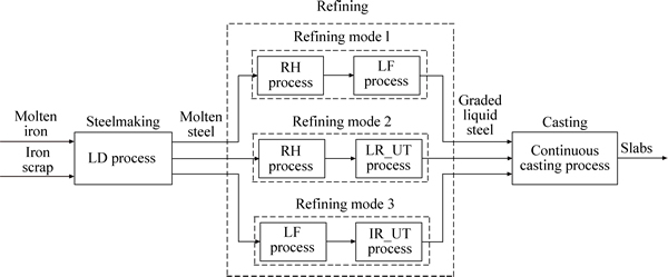
Fig. 1 Steelmaking continuous-casting process
where 


2) Each operation can start only at exactly one particular time.


3) There is an operation precedence constraint in the two consecutive operations of the same job.

where  .
.
4) All jobs in the same batch are processed consecutively in the last stage according to the predefined sequence.


5) A setup time is incurred between two adjacent batches on the same machine in the last stage.

where 


 .
.
6) At a particular time, the number of the jobs simultaneously processed cannot be greater than the total number of units available. This constraint is the machine capacity constraint.


7) The variables must hold for following constraints.


3 Solution methodlogy
Machine capacity relaxation and operation precedence relaxation are commonly used in LR for scheduling problems [15]. In the above model, only machine capacity constraints (5)-(7) couple different jobs on the same machine, so we can relax the constraints to decompose the LR problem into job-level subproblems which can be solved by an efficient DP algorithm. However, the DP algorithm may be time and memory consuming with long time horizons since its computational complexity and multipliers�� number are proportional to the time horizon. On the other hand, if we relax the operation precedence constraints (4), then the LR problem can be decomposed into several single-stage scheduling problems. Although the number of multipliers is proportional to the number of jobs, the single-stage scheduling problems are NP-hard [19]. This implies that full optimization of the subproblems cannot be realized in a reasonable computational time.
Since the full optimization of LR problem is time consuming and spends the majority of the total computational time, the approximate or partial optimization method may be a practical alternative. For the capacity relaxation, the full optimization of all job-level subproblems may be time consuming. The efficiency can be improved significantly by an asymptotical optimization technique presented in Section 4.1. For the precedence relaxation, the NP-hard nature of the LR problem implies that we should find an approximation algorithm for this problem.
3.1 Lagrangian relaxation
Since the derivation and results for the precedence relaxation and capacity relaxation are very similar, we consider the former as follows.
By relaxing the constraints (4) with nonnegative multipliers {��i,g}, we can get the following LR problem.
(LRP) 
where �� is a vector of Lagrangian multipliers {��i,g}; X is the feasible region corresponding to the constraints (2)-(3) and (5)-(9); Ghas been defined previously and

Similarly, the corresponding LD problem is
(LDP) 
subject to

With a given multiplier ��, the LRP problem can be decomposed into single-stage subproblems (LRPj),

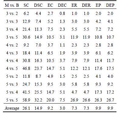
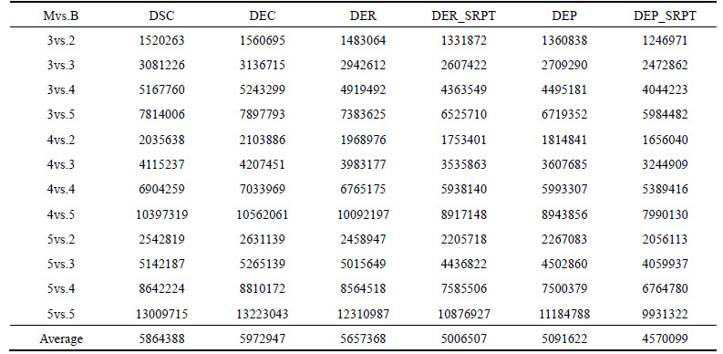
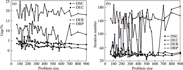
The subproblem for stage j (1��j (LRPj) The subproblem for stage S is give as follows. (LRPS) where For the capacity relaxation, we relax the constraints (5)-(7) and the relaxed problem can be decomposed into |��| job-level subproblems that can be solved by a DP algorithm with the computational complexity proportioned to the time horizon [14]. 3.2 Solution of relaxation problem The subproblem (LRPj) (1��j LENSTRA et al [21] proved that the For the capacity relaxation, the subproblems are job-level scheduling problems, which can be solved by a backward DP with the computational complexity The approximate algorithm for PM and PMR problem are new. We detail them as follows. 3.2.1 Approximation algorithm for PM problem There exists an Thus, the WSPT rule can be applied to get an approximation of the problem Fortunately, the multipliers {��i,g} of the optimal LDP problem make the weights wi,g 3.2.2 Approximation algorithm for PMR problem It is difficult to find an approximate algorithm for the PMR problem with constant approximate ratio like WSPT rule. We propose a two-stage heuristic algorithm based on the WSPT rule. Note that the scheduling method for the jobs with negative weights is the same as the method for the PM problem. For a single-stage scheduling problem, in the first stage, we select the unscheduled jobs whose release times are less than ri+Pi, where the ri is the minimal release time of all unscheduled jobs and Pi is the corresponding processing time. Then, the selected jobs are assigned to the earliest available machine based on the WSPT rule. After scheduling all jobs, the second stage improves all partial schedules on each machine by changing the position of the jobs in each partial schedule to find a better one. It can be known that the computational complexity is 3.3 Construction of a feasible solution to primal problem Since some of the relaxed constraints may not be satisfied, the solution of the dual problem is usually associated with an infeasible schedule. Therefore, a heuristic similar to list scheduling is applied to convert the relaxed schedule into a feasible schedule as follows. For the precedence relaxation, we first substitute the known multipliers into the LR problem. Then, the LR problem becomes a LP problem. The start time of each operation Second, let Finally, since the processing order of jobs on each machine is known, we can get the feasible completion time of each operation {ci,g} by solving an LP problem. Then, we obtain the feasible solution. The feasible construction method of capacity relaxation is similar to that of precedence relaxation. The only difference is the order list (the second step). Specially, let Tj (1�� j 4 Approximate subgradient There are two challenges in LR approach: one is how to optimize the LD problem efficiently, and the other is how to optimize the LR problem efficiently. Since the LD problem is non-differentiable and piecewise affine, it is commonly solved by the subgradient algorithm. However, the convergence of standard subgradient algorithm (SSA) is often very slow because of the so-called zigzagging phenomena [23]. In addition, SSA guarantees the convergence under the strict condition that optimum LD problem is known. On the other hand, the full optimization of the LR problem is time consuming. WANG et al [24] reported that more than 70% of the total solution time is spent on solving the LR problem for job shop scheduling. In order to handle the first challenge, subgradient algorithms with various search-direction strategies have been proposed to weaken the zigzagging phenomena [23, 25]. Additionally, subgradient algorithms with various step-size methods have been developed to replace the strict convergent condition [26, 27], i.e., the optimum should be known a priori. DANTONIO and FRANGIONI [28] tried to combine the two above mentioned techniques to handle the first challenge. To deal with second challenge, ZHAO et al [29] proposed a surrogate gradient algorithm which optimized the LR problem partially. CHEN and LUH [15] adopted this approach to address job scheduling problem. MIJANGOS [30] proposed an approximate subgradient method for nonlinearly constrained network flow problems where the LR problem was asymptotically exact. However, these approaches also face the similar challenge since they use similar subgradient framework. This paper develops existing works to addresses the above two challenges. 4.1 Epsilon-subgradient The standard subgradient algorithm (SSA) for solving the LDP problem is given by where The sub-differential of F at �� is defined as It is easy to see that For the precedence relaxation, it is impossible to get an efficient exact solution of the LR problem because of its NP-hard nature. An alternative way is the approximate algorithm, which can be realized with the methods in Section 3.2. Let F��(��) be an approximate optimization solution of F(��) and For the capacity relaxation, the LR problem can be decomposed into |��| subproblems. It may be time consuming to solve all subproblems per iteration. Indeed, we can optimize asymptotically all subproblems to improve the efficiency by optimizing partial subproblems. Specially, let F(��m, xm) be the value of the m-th iteration and where Obviously, the SSA cannot deal with the above approximate or partial optimization cases. We need to introduce a new subgradient named as epsilon- subgradient. First, we give the definition of the approximately sub-differential of F at �� which is given as follows: and epsilon-subgradient 4.2 Deflected-conditional epsilon-subgradient 4.2.1 Deflected epsilon-subgradient To avoid the interior zigzagging phenomenon, the deflected epsilon-subgradient needs to deflect the subgradient direction whenever it forms an obtuse angle with precious stepping direction phenomenon. Inspired by CAMERINI et al [25], we proposed a modification of the epsilon-subgradient in which the epsilon-subgradient where where There are various forms of the choices of the deflection parameter ��m to ensure that two adjacent subgradients form an acute angle. This work adopts the Camerini-Fratta-Maffioli deflection strategy (CFMDS) Ref. [25] as follows. Proposition 1: Suppose that the deflected epsilon- subgradient where 1<��m<2, then This work selects ��m=1.5 for all m according to the suggestion in Ref. [25]. 4.2.2 Deflected-conditional approximate subgradient algorithm The deflected-conditional epsilon-subgradient (DCES) is first to introduce a feasible approximate subgradient direction, and then deflect the feasible direction to form an acute angle with the precious direction of motion. Finally, the DCES is projected into where 4.3 Deflected-conditional approximate subgradient level algorithm In SSA, the strict convergent condition is difficult to satisfy, namely, the optimum dual function should be known in advance, which cannot be solved in this problem. In order to overcome this shortcoming, an adaptive estimation strategy for the optimum, called Brannlund��s level control strategy [26, 27], is proposed. Inspired by this approach, we introduce the adaptive estimation strategy into the DCASA, resulting in DCASLA as follows. Let P(��) be a primal function value of ��, obtained by the heuristic presented in Section 3.3. Let F��(��) be the approximation of F(��), g��(��) be the conditional approximate subgradient of F(��), and d��(��) be the deflected conditional approximate subgradient of F(��). Denote Step 1: Initialization. Select ��1>0, ��2>0, ��2>0, ��1>0, ��max>0, W>2 (W is an even number), Step 2: Function evaluation. 1) Calculate 2) Calculate P(��m). If Pbest m), set Pbest m). Step 3: Sufficient descent. If Step 4: Small overestimation detection. 1) Set r=r+1, D[r]=F��(��m). 2) If r>W and 3) If r>W, set r=0. Step 5: Large overestimation detection. If Step 6: Updating multipliers. Let Step 7: Accumulation of iterative paths. Set Step 8: Termination check. If Since the deflected-conditional epsilon-subgradient (DCES) is the extension of the standard subgradient, the deflected-conditional approximate subgradient level (DCASL) algorithm generalizes the subgradient level algorithms [27, 28, 30]. 5 Computational experiments 5.1 Algorithm parameters To analyze the performance of the presented algorithms for the SCC scheduling problem, we compare eight methods with different subgradients and relaxation strategies shown in Table 1. Table 1 Meanings of brief notations We denote the SC as the algorithm S adopting the relaxation strategy C. Other seven methods such as DSC, EC, DEC, EP, DEP, ER and DER have similar meanings. The parameters of the DCASL algorithm are provided as follows. ��1=1.0��10-3, ��2=1.0��10-5, t=0.8, W=4, ��=0.8, ��1=(P(��0)+ F(��0))/5, ��max=(P(��0)+F(��0))/||g(��0)||, ��0=0. All algorithms are evaluated with respect to three performance measures: relative duality gap, iteration number, and computational time. Because LR cannot guarantee optimal solutions, the relative duality gap g=(UB-LB)/LB��100% is therefore used as a criterion to measure the solution optimality of the algorithm, where UB is the upper bound derived from the modified feasible solution and LB is the lower bound obtained from the approximate (or exact) solution of LD problem. In addition, let All of the above algorithms are implemented in C# language and run on a PC with Intel Core i7-2600 3.4 GHz 8 GB-CPU using the Windows 7 operating system (64 bit). 5.2 Initialization The initial multipliers should guarantee the non- negativity of the weights of subproblems to avoid redundancy search. Hence, we define the initial iterative multipliers as follows. It is easy to check that the above initial multipliers can make the weights of the subproblems nonnegative. For the capacity relaxation, the initial multipliers are zero (��0=0), which can also guarantee the non- negativity of weights of all subproblems. In addition, the initial time horizon is selected as follows: 5.3 Problem instances Test instances were generated according to the actual production data from Baosteel Complex of China. The problem structures are described as follows. 1) The number of stages is S=4; the number of machines in a stage is chosen from 2) Since there exist only three refining orders (RH->LF, RH->IR_UT and LF_IR_UT) and all jobs in the same batch (any kind of refining order) has same process order, and the processing orders of all batches are generated uniformly in the three given orders. For each pair of the batch and job levels in the combination configurations, we randomly generate 10 instances, resulting in a total of 1��3��4��7��10 = 840 test instances. 5.4 Computational results For simplicity, we denote machines as M, batches as B. Tables 2 and 3 provide the average iteration numbers and average running times of the eight algorithms for each combination of machine and batch, respectively. In each combination of machine and batch, the result of each algorithm is an average from the seven job levels. Table 2 Average iteration numbers of eight algorithms Table 3 Average running times of all algorithms (s) According to the results from Tables 2 and 3, we can get following observations. 1) For the capacity relaxation, the deflected- conditional epsilon-subgradient (DCES) significantly enhances the efficiency of the DCASLA. Namely, the total average iteration number and running time of DEC, which are 44 and 3.0 s respectively, are much better than those of SC, DSC, and EC. In addition, the total average iteration number and running time of DSC are much less than those of SC, which suggests that the deflected- conditional subgradient can also improve the efficiency of the DCASLA when the LR problem is fully optimized. Similar observations can also be found in EC and DEC. On the other hand, although the iteration numbers of EC is much larger than that of SC or DSC, the computational time of EC is less than that of SC or DSC. The reason is that optimizing partially the LR problem per iteration can save much computational time. Nevertheless, it is worth noting that the iteration number of DEC is less than that of SC or DSC, resulting in much less total computational time. 2) For the precedence relaxation, the DCES seems to have no effect on the efficiency of the DCASLA, whereas the tight relaxation strategy makes an obvious improvement in the efficiency. Specially, the differences of iteration number and running time between ER and DER are small, while the iteration number and running time of ER and DER are much less than those of EP and DEP. 3) The running time of DER is much less than that of DEC. This is because the computational complexity of dynamic programming is much higher than that of the WSPT-based heuristic. Interestingly, the iteration number of DER is also less than that of DEC. Tables 4 and 5 provide the average gaps and the average lower bounds of DSC, DEC, DER and DEP. Since the only difference between SC and DSC is the type of subgradient, which implies that SC and DSC have the same solutions. Tables 4 and 5 do not provide the lower bounds of SC. The lower bounds of EC, ER and EP are not provided for the similar reason. The results of DER_SRPT and DEP_SRPT, which are the lower bounds of DEC and DEP, are obtained based on the SRPT rule in Section 3.3. In addition, Fig. 2 depicts the average duality gaps and iteration numbers of four algorithms at various problem sizes that are equal to 1) The overall average gap of DEC is the smallest among four algorithms, 2.70%. In addition, the overall average lower bound of DEC is also the best. Since DEC adopts asymptotical optimization strategy, the lower bound may be larger than the optimal lower bound. Nevertheless, Table 5 shows that the differences of lower bounds generated by DEC and DSC are small. This suggests that the lower bound of DEC is very close to the optimal lower bound since DSC adopts full optimization strategy. 2) The comparisons among the four algorithms in Tables 4-5 and Fig. 2 show that the iteration number and gap of DEC are the least. It is worth noting that the iteration number and gaps of DER fluctuate wildly with the increasing of problem scale. This suggests that DEC is more robust than DER. 6 Conclusions To solve a real-world FJS-type SCC scheduling problem, this paper presented a LR approach with two relaxation strategies, i.e., machine capacity relaxation and operation precedence relaxation, based on a time- index formulation. We obtained a highly efficient LR framework by optimizing partially LR problems and employing a generalized SSA, named as DCASLA, to solve LD problems. Computational experiments demonstrated that the proposed methods could generate a high quality solution within an acceptable time. Table 4 Average gaps of four algorithms (%) Table 5 Average lower bounds of four algorithms Fig. 2 Comparisons of gaps (a) and iteration numbers (b) of four algorithms The efficiency and effectiveness of DCASLA were investigated by adopting different types of subgradients and relaxation strategies. For the precedence relaxation, the LR problem is optimized approximately. Computational results showed that the tighter relaxation strategy could not only improve the solution quality but also enhance the efficiency of DCASLA significantly. Nevertheless, the type of subgradient had little influence on the efficiency. For the capacity relaxation, the asymptotical optimization technique improved the efficiency of DCASLA dramatically. Notation Indices, sets, and number of elements Mj Number of machines available at the j-th stage s(i, g) The stage that is visited by the the g-th operation of job i �� Set of indices of all jobs, |��| is the number of all jobs ��n Set of indices of the n-th batch, Bk Set of indices of all batches on the k-th machine at last stage s(n) Index of the last job in the n-th batch, b(k) Index of the last batch on the k-th machine in the last stage, Data or fixed parameters Pij Processing time of job i at stage j Tj,j+1 Transportation time from stage j to stage j+1 Su Setup time between two adjacent batches on the same machine in the last stage W1 Penalty coefficient for the sojourn time of each job W2 Penalty coefficient for the completion time of each job in stage S T Total number of time periods in the planning horizon Decision variables xi,g,t 0/1 variable that is equal to one if and only if the g-th operation of job i starts at time period t ci,g Completion time of the g-th operation of job i References [1] TANG Li-xin, WANG Gong-shu. Decision support system for the batching problems of steelmaking and continuous-casting production [J]. Omega-International Journal of Management Science, 2008, 36(6): 976-991. [2] PACCIARELLI D, PRANZO M. Prodution scheduling in a steelmaking-continuous casting plant [J]. Computers and Chemical Engineering, 2004, 28(12): 2823-2835. [3] BELLABDAOUI A, TEGHEM J. A mixed-integer linear programming model for the continuous casting planning [J]. International Journal of Production Economics, 2006, 104(2): 260-270. [4] KUMAR V, KUMAR S, CHAN F T S, TIWARI M K. Auction-based approach to resolve the scheduling problem in the steelmaking process [J]. International Journal of Production Research, 2006, 44(8): 1503-1522. [5] MISSBAUER H, HAUBERB W, STADLER W. A scheduling system for the steelmaking-continuous casting process: A case study from the steelmaking industry [J]. International Journal of Production Research, 2009, 47(15): 4147-4172. [6] ATIGHEHCHIAN A, BIJARI M, TARKESH H. A novel hybrid algorithm for scheduling steelmaking continuous casting production [J]. Computers & Operations Research, 2009, 36(8): 2450-2461. [7] PANG Quan-ke, WANG Ling, MAO Kun, ZHAO Jin-hui, ZHANG Min. An effective artificial bee colony algorithm for a real-world hybrid flowshop problem in Steelmaking process [J]. IEEE Transactions on Automation Science and Engineering, 2013, 10(2): 307-322. [8] TAN Yuan-yuan, HANG Ying-lei, LIU Shi-xin. Two-stage mathematical programming approach for steelmaking process scheduling under variable electricity price [J]. International Journal of Iron and Steel Research, 2013, 27(7): 1-8. [9] YE Yun, LI Jie, LI Zu-kui, TANG Qiu-hua, XAO Xin, Christodoulos A. Floudas. Robust optimization and stochastic programming approaches for medium-term production scheduling of a large-scale steelmaking continuous casting process under demand uncertainty [J]. Computer and Chemical Engineering, 2014, 66: 165-185. [10] MAO Kun, PAN Quan-ke, PANG Xin-fu, CHAI Tian-you. A novel Lagrangian relaxation approach for the hybrid flowshop scheduling problem in a steelmaking-continuous casting process [J]. European Journal of Operational Research, 2014, 236(1): 51-60. [11] HAO Jing-hua, LIU Min, JIANG Sheng-long, WU Cheng. A soft-decision based two-layered scheduling approach for uncertain steelmaking-continuous casting process [J]. European Journal of Operational Research, 2015, 244(3): 966-979. [12] WANG Gui-rong, LI Qi-qiang, WANG Lu-hao. An improved cross entropy algorithm for steelmaking-continuous casting production scheduling with complicated technological routes [J]. Journal of Central South University, 2015, 22(8): 2998-3007. [13] HMIDA A B, HAOUARI M, HUGUET M J, LOPEZ P. Discrepancy search for the flexible job shop scheduling problem [J]. Computers and Operations Research, 2010, 37(12): 2192-2201. [14] CHEN H, CHU C, PROTH J M. An improvement of the Lagrangian relaxation approach for job shop scheduling: a dynamic programming method [J]. IEEE Transactions on Robotics and Automation, 1998, 14(5): 786-795. [15] CHEN H, LUH P B. An alternative framework to Lagrangian relaxation approach for job shop scheduling [J]. European Journal of Operational Research, 2003, 149(3): 499-512. [16] NISHI T, HIRANAKA Y, INUIGUCHI M. Lagrangian relaxation with cut generation for hybrid flowshop scheduling problems to minimize the total weighted tardiness [J]. Computers & Operations Research, 2010, 37(1): 189-198. [17] TANG Li-xin, LUH P, LIU Ji-yin, FANG Lei. Steelmaking process scheduling using Lagrangian relaxation [J]. International Journal of Production Research, 2002, 40(1): 55-70. [18] XUAN Hua, TANG Li-xin. Scheduling a hybrid flowshop with batch production at the last stage [J]. Computers & Operations Research, 2007, 34(9): 2718-2733. [19] TANG Li-xin, XUAN Hua, LIU Ji-yin. A new Lagrangian relaxation algorithm for hybrid flowshop scheduling to minimize total weighted completion time [J]. Computers & Operations Research, 2006, 33(11): 3344-3359. [20] BRUNO J. GOFFMAN E, SETHI R. Scheduling independent tasks to reduce mean finishing time [J]. Communications of the ACM, 1974, 17(7): 382-387. [21] LENSTRA J K, KAN A.H.G, BRUKER P. Complexity of machine scheduling problems [J]. Annals of Discrete Mathematics, 1977, 7(1): 343-362. [22] KAWAGUCHI T, KYAN S. Worst case bound of an LRF schedule for the mean weighted flow time problem [J]. SIAM Journal of Computing, 1986, 15(4): 1119-1129. [23] GUTA B. Subgradient optimization methods in integer programming with an application to a radiation therapy problem [D]. Kaiserlauter: Teknishe Universitat Kaiserlautern, 2003. [24] WANG Jia-hua., LUH P B, ZHAO Xing. An optimization-based algorithm for job shop scheduling [J]. Sadhana, 1997, 22(2): 241-256. [25] CAMERINI P M, FRATTA L, MAFFIOLI F. On improving relaxation methods by modified gradient techniques [J]. Mathematical Programming Study, 1975, 3: 26-34. [26] BRANNLUND U. On relaxation methods for nonsmooth convex optimization [D]. Stockholm, Sweden: Royal Institute of Technology, 1993. [27] GOFFIN J L, KIWIEL K C. Convergence of a simple subgradient level method [J]. Mathematical Programming, 1999, 85(1): 207-211. [28] D'ANTONIO G, FRANGIONI A. Convergence analysis of deflected-conditional approximate subgradient methods [J]. SIAM Journal on Optimization, 2009, 20(1): 357-386. [29] ZHAO Xing, LUH P B, WANG Jian-hua. Surrogate gradient algorithm for Lagrangian relaxation [J]. Journal of Optimization Theory and Applications, 1999, 100(3): 699-712. [30] MIJANGOS E. Approximate subgradient methods for nonlinearly constrained network flow problems [J]. Journal of Optimization Theory and Applications, 2006, 128(1): 167-190. (Edited by DENG L��-xiang) Cite this article as: PANG Xin-fu, GAO Liang, PAN Quan-ke, TIAN Wei-hua, YU Sheng-ping. A novel Lagrangian relaxation level approach for scheduling steelmaking-refining-continuous casting production [J]. Journal of Central South University, 2017, 24(2): 467-477. DOI: 10.1007/s11171-017-3449-9. Foundation item: Projects(51435009, 51575212, 61573249, 61371200) supported by the National Natural Science Foundation of China; Projects(2015T80798, 2014M552040, 2014M561250, 2015M571328) supported by Postdoctoral Science Foundation of China; Project(L2015372) supported by Liaoning Province Education Administration, China Received date: 2015-11-13; Accepted date: 2016-01-13 Corresponding author: PANG Xin-fu, PhD; Tel: +86-17702400935; E-mail: pangxinfu@163.com


 (1
(1
 problem is NP-hard, and proved that
  is a strongly NP-hard problem. Nevertheless, we can use the approximation algorithm to solve the problems.
 [14].
[14]. -approximate algorithm for the PM problem of which the weights are nonnegative [22].This algorithm is also called WSPT rule. However, some weights of the PM problem may be negative during the iterations of subgradient algorithms. We need to generalize the approximate algorithm for PM problems with any weights. Let

 It is easy to see that the completion time of jobs in
  should be as large as possible so as to minimize the objective. Hence, the scheduling of jobs in
  starts at time zero, while the scheduling of jobs in completes at end of time horizon T. This implies that we can schedule two kinds of jobs in two disjoint time intervals because of
 For the jobs in
  we can apply directly WSPT rule to get approximate solution. For the jobs in
  we also can use WSPT rule but need some transformation. Let
  and
and 
 then
then (15)
(15) where the processing time of job i is
 1��j
1��j
 can be obtained by solving the LP problem.
 (1��g
(1��g and Tj (1��j
 Assign the job to the earliest available machine at stage j according to the list Tj (1��j
 Assign the job to the earliest available machine at stage j according to the list Tj (1�� j
 m=0, 1, 2, �� (16)
 g(��m) is the subgradient of F(��m), F(��m)=-LRP(��m);
  �� is the corresponding multiplier with inequality constraints such as the precedence constraints (4) and n1 is the number of inequality constraints.
 (17)
(17) From Eq. (16), a new subgradient direction is obtained by optimizing fully the LR problem.
 be its lower bound, then
  and
and 
 be the new multiplier, and then we only need to find an xm+1 such that
 corresponds to the i-th subproblem
  This is easy to be realized since we can optimize each subproblem and compare it with from i=1 to i=|��|. Once there exists an
 such that
  , then we find the required xm+1 and stop searching. This implies that there exists an error
  If such an xm+1 cannot be obtained, xm+1=xm, which implies the error ��=0.
 (18)
(18) If ��=0, then g��(��) becomes the standard subgradient g(��). The recursive equation of the approximate subgradient algorithm (ASA) is the same as that of standard subgradient algorithm in Eq. (16) except that the g(��) is replaced with the g��(��). Similar approximate ideas can also be found in Ref. [29]. They introduced a surrogate subgradient to represent the new subgradient obtained without full optimization. The surrogate subgradient can thus be viewed as an epsilon-subgradient.
 at an iterate ��m is replaced by a deflected epsilon- subgradient
  given by
 is a suitable scale called a deflection parameter and
  for m=0. So, the deflected approximate subgradient algorithm (DASA) for the LD problem is
 (19)
(19) m=0, 1, 2, �� (20)is the approximate subgradient of F(��m) at ��m.
 is given by the DASA, the step length ��m>0 and the deflection parameter ��m is given by
 (21)
(21) This means that the two consecutive epsilon-subgradients generated by the DASA form an acute angle.
 to get a feasible direction. Thus, we can obtain a deflected-conditional approximate subgradient algorithm (DCASA) as follows:
 (22)
(22) (23)
(23) , m=0, 1, 2, �� (24)
 is the conditional epsilon-subgradient of F(��m) at ��m and ��m��0 is the deflection parameter.
 and
and 

 Set ��best=��0, r>0, ��1>0,
  m=0, l=1, s=0,
  , M[l]=1 (M[l] will denote the iteration number when the l-th update of
  occurs). Calculate P(��0) and set Pbest=P(��0). Denote h(s)=1/(s+1).
 If
If set
set 
 Otherwise, set
 then set
  ��m=0, ��l+1=��l, and l=l+1.
 set
set 


 m=m1.
m=m1. , then ��m=��best, ��m=0, dm-1=0, ��l+1=�¦�l , l=l+1, s=s+1.
 Calculate
 Update multipliers as Eqs. (22)�C(23), where

 m=m+1.
 or
or  is satisfied, stop iteration; otherwise, go to Step 2.
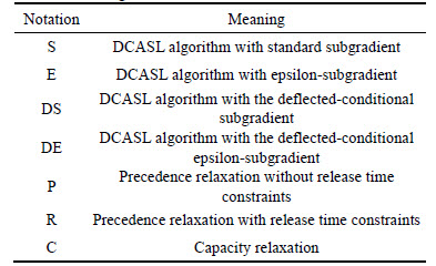
 where
where  is the lower bound of LD problem obtained by the SPRT rule in the precedence relaxation.


 where
where  is the largest value of the feasible solution P(��0) obtained from the construction method in Section 3.3, and
 .
. (1��j��S); the number of batches is chosen from
  (1��k��MS); the number of jobs in a batch is chosen from
  for all n; the penalty coefficients is W1=10, W2=10+20(S-1) and the setup time is Su=80. The integer of the transportation time Tj,j+1 is generated uniformly in the range of [3, 10]. The integer of the processing time Pi,j is generated uniformly in the range of [36, 50].
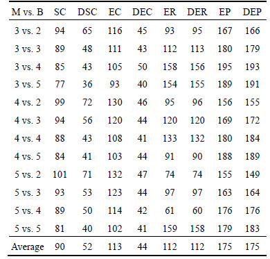
 Some observations are provided as follows.
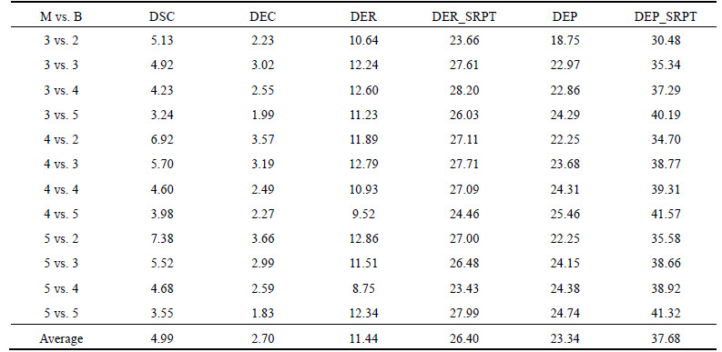
 ,
,  where N is the total number of batches.
  for any
  and
and 

 s(0)=0, s(N)=|��|,


 b(0)=0, b(Ms)= N, 1��k��Ms, where S is the total number of stages. Then,

