ARTICLE

J. Cent. South Univ. (2019) 26: 2119-2128

DOI: https://doi.org/10.1007/s11771-019-4159-7

Simulation of alumina dissolution and temperature response under different feeding quantities in aluminum reduction cell

LI Si-yun(李斯昀), LI Mao(李茂), HOU Wen-yuan(侯文渊),LI He-song(李贺松), CHENG Ben-jun(程本军)

School of Energy Science and Engineering, Central South University, Changsha 410083, China

Central South University Press and Springer-Verlag GmbH Germany, part of Springer Nature 2019

Abstract: In the feeding process of aluminum electrolytic, feeding quantity of alumina affects eventually dissolved quantity at the end of a feeding cycle. Based on the OpenFOAM platform, dissolution model coupled with heat and mass transfer was established. Applying the Rosin-Rammler function, alumina particle size distribution under different feeding quantities was obtained. The temperature response of electrolyte after feeding was included and calculated, and the dissolution processes of alumina with different feeding quantities (0.6, 0.8, 1.0, 1.2, 1.4, 1.6 kg) after feeding were simulated in 300 kA aluminum reduction cell. The results show that with the increase of feeding quantity, accumulated mass fraction of dissolved alumina decreases, and the time required for the rapid dissolution stage extends. When the feeding quantity is 0.6 kg and 1.2 kg, it takes the shortest time for the electrolyte temperature dropping before rebounding back. With the increase of feeding quantity, the dissolution rate in the rapid dissolution stage increases at first and then decreases gradually. The most suitable feeding quantity is 1.2 kg. The fitting equation of alumina dissolution curve under different feeding quantities is obtained, which can be used to evaluate the alumina dissolution and guide the feeding quantity and feeding cycle.

Key words: alumina dissolution; heat and mass transfer; particle size distribution; temperature response; numerical simulation

Cite this article as: LI Si-yun, LI Mao, HOU Wen-yuan, LI He-song, CHENG Ben-jun. Simulation of alumina dissolution and temperature response under different feeding quantities in aluminum reduction cell [J]. Journal of Central South University, 2019, 26(8): 2119-2128. DOI: https://doi.org/10.1007/s11771-019-4159-7.

1 Introduction

In aluminum electrolysis production, the dissolution and diffusion rate of the main raw material alumina directly determines the stability of electrolysis process [1]. If the alumina particles accumulate, the surrounding alumina concentration is overly higher, or the electrolyte temperature is too low due to excessive local heat absorption, the alumina will form agglomerates, and the undissolved agglomerates will form a precipitate (soft mud) and shell on the surface of the cathode. Especially in the 300 kA and 500 kA aluminum reduction cell, the anode-cathode distance (ACD) is gradually reduced, the dissolution and diffusion of alumina is more difficult, and the agglomerates cannot be dissolved in time and precipitate to the bottom of the cell. How to ensure that alumina can be dissolved and diffuse rapidly in the electrolyte after feeding is an urgent problem to be solved.

In order to study the dissolution process of alumina in the actual reduction cell, YANG et al [2] and QIU et al [3] studied the behavior of alumina dissolution after adding it to the electrolyte in a quartz transparent cell, and found that there are three stages of alumina dissolution. XU et al [4] tested the dissolution rate of alumina and found that preheating alumina and increasing the superheat of electrolyte can significantly increase the dissolution rate of alumina. The data from the “Testing device for determining alumina dissolution” by WALKER [5] showed that the alumina concentration of the cell grows at the same rate as the feed rate, i.e., no precipitation occurs when the alumina dissolves rapidly. WELCH et al [6] found through experiments that the dissolution process of alumina can be divided into two stages: rapid dissolution stage and slow dissolution stage, that is, part of alumina with good dispersion is rapidly dissolved, while the aggregated alumina forms agglomeration and is slowly dissolved. From the dissolution mechanism of alumina, POI et al [7] and VERHAEGHE et al [8] believed that the driving force of alumina dissolution is the difference in alumina concentration, so as to propose a mass transfer model of alumina dissolution. LILLEBUEN et al [9] and BEREZIN et al [10] considered that superheat is the main driving force of alumina dissolution, and proposed a heat transfer model for alumina dissolution. TAYLOR et al [11] predicted that 400 μm can be used as the characteristic size to identify the control mechanism of dissolution based on experiments. In the study of HOU et al [12], two kinds of dissolution control mechanisms such as heat transfer and mass transfer were studied and analyzed in detail. Based on the dimensionless heat and mass transfer equations, the critical diameter 520 μm is proposed to determine the dominant mechanisms. ZHAN et al [13] and ZHANG [14] studied the effect of anodic gas bubbles and electromagnetic force on the dissolution and diffusion process of alumina in actual aluminum reduction cell, and found that the effect of bubbles on the alumina dissolution is more important.

Although there are many researches on the mechanism and process of alumina dissolution, there are few studies on the alumina feeding quantity in actual electrolytic production. Especially for small cell of 160 kA or large cell of 500 kA, the signal feeding quantity is all 1.8 kg. Whether the 1.8 kg feeding quantity is optimal is still a question. In addition, the dissolution characteristic curve of alumina in the actual reduction cell has not been studied, and this characteristic curve is of guiding significance to the control of alumina feeding.

In this work, based on the calculation platform of OpenFOAM, a self-programming module coupling the dissolution of alumina under heat transfer and mass transfer, electrolyte flow, particle motion and temperature response in aluminum reduction cell was developed. The Rosin-Rammler distribution function was used to obtain the particle size distribution of alumina under different feeding quantities. Numerical simulation was conducted for the dissolution process of alumina particles in actual 300 kA aluminum reduction cell under different feeding quantities. The change of the cumulative dissolved mass percentage of alumina and the electrolyte temperature response in the feeding zone within a feeding cycle were studied to obtain the optimal feeding quantity. On this basis, the dissolution characteristic curves under different feeding quantities can be obtained, and the dissolution equation was obtained by fitting, which can provide theoretical guidance for evaluating the alumina dissolution and guiding the feeding quantity and feeding cycle.

2 CFD modeling

2.1 Physical model

2.1.1 Physical parameters

The 300 kA aluminum reduction cell was used as the research object, and the dissolution process of the alumina in the reduction cell was simulated. The specific cell parameters are shown in Table 1.

2.1.2 Computational region

In this work, the 300 kA aluminum reduction cell is taken as the research object, and the bubble is the main driving force for dispersing the alumina particles. The electrolyte flow field under the action of bubbles is symmetric about the long axis and the short axis. Without affecting the accuracy of the calculation and in order to reduce the calculation cost, the half-cell was selected to simulate the dissolution process of alumina under the action of bubbles.

The half-cell size is 3840 mm×7400 mm×180 mm. The calculation region and the feeding zone are shown in Figures 1 and 2.

Table 1 Physical parameters of aluminum reduction cell

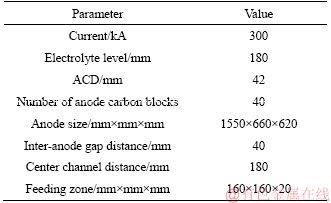
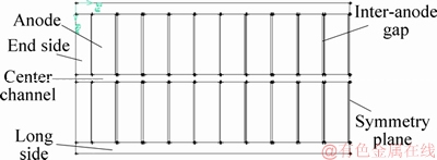
Figure 1 Calculation region of aluminum reduction cell

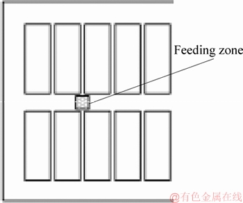
Figure 2 Schematic diagram of alumina feeding zone

2.1.3 Basic assumption

In the actual aluminum electrolysis process, the dissolution process of alumina particles is affected by many factors, and the following assumptions are made during the simulation calculation [15]:

1) Ignore the consumption of the anode carbon block and maintain the level of the anode bottom palm.

2) Ignore the influence of the ledge.

3) Ignore the effect of the aluminum layer on the movement of the electrolyte.

4) The formation process of agglomerates is neglected.

5) Ignore the consumption of alumina in the electrolyte and the heating of the electrolyte by current, focusing on the dissolution process of alumina.

2.2 Mathematical model

2.2.1 Alumina particle dissolution model

The dissolution of alumina is controlled by two dissolution mechanisms of heat transfer and mass transfer. It is found that the dissolution of alumina particles less than 520 μm is controlled by mass transfer mechanism, and the dissolution of alumina particles larger than 520 μm is controlled by heat transfer mechanism. The mass transfer and heat transfer dissolution model has been established in our previous work and its derivation process can be found in Refs. [12, 16].

Under the mass transfer control mechanism, the shrinking sphere model of alumina particles is expressed as follows:

                       (1)

Under the heat transfer mechanism, the shrinking sphere model of alumina particles is as follows:

             (2)

where k is the mass transfer coefficient, m/s; h is the convection heat transfer coefficient, W/(m²·K); C_Al is specific heat capacity of alumina, J/(kg·K); ΔH_diss is heat of dissolution for alumina, J/kg; r_L is the density of electrolyte, kg/m³; r_S is density of alumina particle, kg/m³; c_sat is the saturation concentration of alumina in electrolyte, %; c is the local alumina concentration, wt%; T_L is the temperature of electrolyte, K; T_liq is the liquidus temperature of electrolyte, K.

In fact, the critical diameter is related to the environment where the particles are located, including electrolyte temperature, superheat and alumina concentration around the particles. The critical diameter obtained is an approximate value. In order to calculate more accurately, the dissolution rate under the two mechanisms of heat transfer and mass transfer is first calculated in the simulation, then the dissolution rate under the two mechanisms is compared. The slow dissolution rate, which is the rate-controlling step [12], is computed and selected as the dissolution rate of alumina in each simulation step.

2.2.2 Momentum equation

For the electrolyte flow under the action of bubbles, it is mainly affected by the bubble force and the drag force between the alumina particles and the electrolyte, which satisfies the following momentum equation:

    (3)

     (4)

  (5)

where t is time, s; u_L is the velocity vector of electrolyte, m/s; m is the effective viscosity of electrolyte, kg/(m·s); u, v and w represent the components of the velocity vector u_L in the x, y, and z directions, respectively, m/s; S is a generalized source term, including volume force, bubble force, and particle-electrolyte momentum exchange term S_m, etc., where S_m is as follows:

    (6)

where V_cell is the unit grid volume, m³; F_D is drag force on alumina particle, N; u_P is the particle velocity, m/s.

2.2.3 Drag model

In most fluid-particle two-phase flow, the drag force is the main force acting on the particles. The magnitude of the drag is related to the particle size, the relative velocity between the particle and the fluid, as well as the drag coefficient. The drag formula is as follows [17]:

              (7)

where A_p=πd_p²/4, represents the cross-sectional area of alumina particles, m²; C_D is the drag force coefficient, which is related to the Reynolds number of alumina particles, and is expressed as follows:

 (8)

Lagrange method is always used to track the movement of alumina particles. Through the force analysis of a single particle, Newton’s second law is applied:

                                (9)

                 (10)

2.2.4 Transport model

After the alumina particles are dissolved into the electrolyte, the transport equation for the alumina concentration is established as follows:

        (11)

where Γ_c is the diffusion coefficient of alumina, m²/s; S_c is the dissolved mass in unit time per cell.

The dissolution process of alumina in the electrolyte is an endothermic process, which causes the electrolyte temperature drop. The energy equation is established as follows:

  (12)

where l is the thermal conductivity, W/(m×K); S_T is the heat absorption in unit time per cell.

2.3 Calculation condition

In this paper, 300 kA aluminum reduction cell is used as the research object, and one of the feeding points (as shown in Figure 2) is selected for alumina feeding. The feeding quantities are 0.6, 0.8, 1.0, 1.2, 1.4 and 1.6 kg, respectively. Since the calculation of the bubble-electrolyte-particle three- phase is difficult, the flow of the electrolyte under the action of the bubbles is first calculated using CFX. Then, the bubble force on electrolyte is extracted and added in momentum equation as the source term to calculate the electrolyte flow field, so as to obtain the movement of alumina particles, the dissolution and transport process of alumina, as well as the distribution of alumina concentration and electrolyte temperature.

3 Multi-particle dissolution under Rosin- Rammler distribution

3.1 Liquidus temperature

For electrolytes, the liquidus temperature is related to the electrolyte component content, such as AlF₃, Al₂O₃, MgF₂, and CaF₂. The empirical formula, obtained by ZHANG et al [18] and HOU [19] using the experimental results for regression calculation, is used to calculate the liquidus temperature. The formula is expressed as follows:

　      (13)

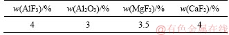
The initial electrolyte composition selected in this paper is shown in Table 2. After calculation, the initial liquidus temperature is 950 °C.

Table 2 Electrolyte composition [20]

3.2 Electrolyte flow field under action of bubbles

The bubble force in 300 kA aluminum reduction cell calculated in our previous work is extracted [21] and added in the electrolyte momentum equation as the source term. The electrolyte flow field obtained is shown in Figure 3.

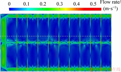
Figure 3 Electrolyte flow field under action of anode bubbles

It can be clearly seen from Figure 3 that the maximum flow rate of the electrolyte under the action of the anodic bubble is 0.55 m/s. The feeding zone is located at the junction between the inter-　anode gap and the center channel, where the electrolyte flow velocity is high. The electrolyte in the two inter-anode gap flows into the center channel which makes the electrolyte stir up and down and is conducive to the rapid dispersion and dissolution of alumina particles.

3.3 Particle size distribution with　different feeding quantities

The size of the feeding zone is 16 cm×16 cm× 2 cm, and a total of 128 grids are generated. Therefore, 128 particles are fed at each time step (0.001 s), and the whole time of feeding is 0.1 s. The number of particles after feeding will represent the total number of alumina particles added to the actual reduction cell. The Rosin-Rammler (R-R) distribution function of alumina particles in the electrolyte after feeding is as follows [19]:

R=100e^-0.0154x0.65                         (14)

The alumina particles have a particle size in the range of 40 μm to 200 μm before adding into the electrolyte, and most of the particles are concentrated in about 100 μm. Once added in the electrolyte, some of the alumina particles are encapsulated by the solidified electrolyte to form agglomerated particles. In actual production, the maximum agglomerated particle size is generally between 1 and 1.5 cm [22]. When simulating the actual dissolution of alumina particles, since the simulation cannot be carried out according to the actual alumina particle size, it is best to select a representative particle size as the characteristic particle size according to R-R distribution. When calculating, the maximum agglomerate particle size is 1 cm, and the final selected characteristic particle size distribution is shown in Table 3.

Table 3 Particle size distribution after feeding

The number of alumina particles added to the actual aluminum reduction cell is hundreds of millions. The current numerical simulation is far from the calculation requirement, so it is necessary to rationally simplify the number of alumina particles. An alumina particle is used to represent a certain number of actual alumina particles. When calculating the alumina concentration, the actual dissolved mass is that a single particle dissolved mass multiplying by the number of particles that it represents. The calculation method of temperature field is the same.

3.4 Analysis of alumina dissolution with different feeding quantities

The simulation is carried out for the feeding quantity from 0.6 kg to 1.6 kg, and the percentage of cumulative dissolved mass of alumina within one cycle is shown in Figure 4. With comparing the results of the cumulative dissolved mass percentage of different quantities, it can be seen that with the increase of the feeding quantity, the percentage of the final cumulative dissolved mass gradually decreases at the end of a feeding cycle, that is, the final undissolved total quantity of alumina particles is increased and the dissolution efficiency is lowered. KOBBELTVEDT [23] found that half quantity of alumina dissolves within 15 s, and this period is defined as the rapid dissolution stage. It can be seen from Figure 4 that the time required for the alumina to dissolve half percent is about 14, 16, 17, 17, 19.5, 21 s, that is, as the feeding quantity increases, the time period required for the rapid dissolution of alumina gradually increases. Figure 5 shows the calculation of the dissolution rate in rapid dissolution stage with different feeding quantities. It can be seen from the figure that in the mass range of 0.6-1.2 kg, the dissolution rate of alumina increases rapidly with the increase of mass, while in the range of 1.2-1.6 kg, the dissolution rate changes little. This is mainly due to the fact that when the feeding quantity is low, the dissolution only has little effect on the alumina concentration and the superheat of the electrolyte, and particles with good dispersion can be dissolved quickly. With the increase of mass, the difference of alumina concentration and the superheat of electrolyte decrease, which restricts the dissolution of alumina particles, resulting in the decrease of dissolution rate.

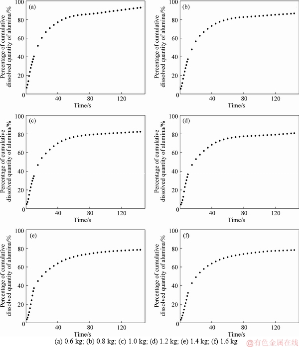
Figure 4 Cumulative dissolved mass percentage of alumina with different quantities:

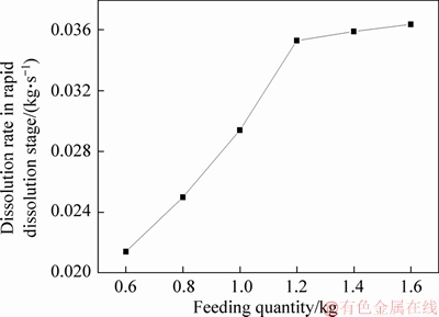
Figure 5 Dissolution rate in rapid dissolution stage with different feeding quantities

From the analysis of the percentage of cumulative dissolved quantity and dissolution rate of alumina, it can be seen that when the feeding quantity is 1.2 kg, the dissolution rate basically reaches the maximum, and the cumulative dissolved quantity is more than 80%. If the feeding quantity is more than 1.2 kg, although the dissolution rate is basically the same, there are too many undissolved agglomerates which are easy to form precipitation. However, if the feeding quantity is less than 1.2 kg, the dissolution rate is lower, which can easily lead to the low alumina concentration in electrolytes. Thus, the most suitable feeding quantity is 1.2 kg.

3.5 Analysis of electrolyte temperature change in feeding zone

After adding alumina into the electrolyte from the feeding zone, the electrolyte temperature in the feeding zone drops obviously. Figure 6 shows the average temperature change of the electrolyte in the feed zone with 0.6, 0.8, 1.0, 1.2, 1.4 and 1.6 kg, respectively.

It can be seen from Figure 6 that after the alumina particles entering the feeding zone, the dispersed small particles dissolve rapidly and absorb a large quantity of heat, and the electrolyte temperature drops rapidly from the initial temperature of 1233 K (960 °C). Comparing the curves in Figure 6, the time for the electrolyte temperature dropping to the lowest temperature is 22, 30, 30, 24, 32 and 28 s, respectively. When the feeding quantity is 0.6 kg and 1.2 kg, it takes the shortest time for the electrolyte temperature dropping before rebounding back. Under the action of bath flow and heat transfer, the temperature of electrolyte in feeding zone rebounds back slowly by the supplement of the surrounding high temperature electrolyte.

After the alumina is added to the electrolyte, the cold alumina absorbs heat from the electrolyte. At the same time, the dissolution of alumina is also an endothermic process. When the electrolyte temperature drops below the liquidus temperature, the electrolyte solidifies, and the poorly dispersed alumina is wrapped by the solidified electrolyte to form agglomerates, which will only dissolve when heated to the electrolyte temperature.

3.6 Fitting curve of alumina dissolution characteristics

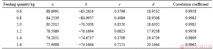
Fitting curves are usually used to describe characteristic laws [24, 25]. According to the percentage of cumulative dissolved alumina mass under different feeding quantities, the fitting curve can be obtained by fitting, as shown in Figure 7. The fitting function is expressed by Formula (15), and the corresponding parameters are shown in Table 4. According to the correlation coefficients of the fitting results, they are all larger than 0.995, indicating that the fitting function meets the requirements.

                         (15)

At present, the feeding control of aluminum reduction cell is mainly controlled and operated according to the voltage fluctuation, and the criterion to conduct feeding is simplified and plausible, which may easily lead to overfeeding or underfeeding. According to the dissolution function of alumina under different feeding quantities obtained in this work, the dissolution of alumina can be effectively estimated and under control.

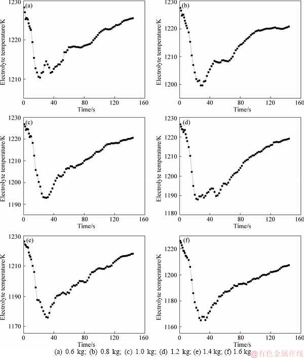
Figure 6 Average temperature curve of electrolyte in feeding zone:

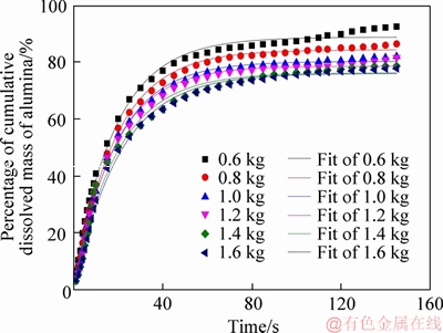
Figure 7 Fitting curve of alumina dissolution characteristics under different feeding quantities

4 Conclusions

Based on the OpenFOAM platform, the calculation module coupling the alumina dissolution under heat and mass transfer, electrolyte flow, alumina diffusion and temperature response in aluminum reduction cell was developed. The alumina particle size distribution under different feeding quantities was obtained using the Rosin-Rammler distribution function. The dissolution process of alumina particles in the actual 300 kA aluminum reduction cell under different feeding quantities was numerically simulated. Based on the simulation and discussions, the following conclusions can be drawn:

Table 4 Corresponding parameters of fitting curves under different feeding quantities

1) With the increase of the feeding quantity, the mass percentage of the final cumulative dissolved alumina gradually decreases at the end of a feeding cycle, and the time required for the alumina to dissolve half quantity gradually increases, which is about 14, 16, 17, 17, 19.5 and 21 s, respectively. The time required for the electrolyte temperature dropping before rebounding back is the shortest when the feeding quantity is 0.6 kg and 1.2 kg.

2) In the mass range of 0.6-1.2 kg, the dissolution rate of alumina increases rapidly with the increase of mass, while in the range of 1.2-1.6 kg, the dissolution rate changes little. With the increase of feeding quantity, the dissolution rate in the rapid dissolution stage increases at first and then decreases gradually. Considering the percentage of cumulative dissolved mass and dissolution rate of alumina, it can be drawn that the most suitable feeding quantity is 1.2 kg.

3) By fitting the dissolution characteristic curve of alumina, the fitting equation under different feeding quantities is obtained, which can be expressed as y=a+b·e^(c-x)/d. The correlation coefficients are all greater than 0.995. The fitting function can be used to evaluate the alumina dissolution and guide the feeding quantity and feeding cycle.

References

[1] YANG You-jian, GAO Bing-liang, WANG Zhao-wen, SHI Zhong-ning, HU Xian-wei. Effect of physiochemical properties and bath chemistry on alumina dissolution rate in cryolite electrolyte [J]. JOM, 2015, 67(5): 973-983. DOI: 10.1007/s11837-015-1379-7.

[2] YANG Zhen-hai, GAO Bing-liang, XU Ning, QIU Zhu-xian, LIU Yao-kuan. Dissolution of alumina in molten cryolite (photogrammetry) [J]. Journal of Northeastern University, 1999, 20(4): 398-400. DOI: 10.3321/j.issn:1005- 3026.1999.04.017. (in Chinese)

[3] QIU Zhu-xian, YANG Zhen-hai, GAO Bing-liang, XU Ning, LIU Yao-kuan. Dissolution of alumina in molten cryolite (A video recording study) [C]// ECKERT CE Light Metals 1999. San Diego, CA: TMS, 1999: 467-471.

[4] XU Jun-li, SHI Zhong-ning, GAO Bing-liang, QIU Zhu-xian. Dissolution of alumina in melted cryolite [J]. Journal of Northeastern University, 2003, 24(9): 832-834. DOI: 10.3321/j.issn:1005-3026.2003.09.005. (in Chinese)

[5] WALKER D I. Alumina in aluminum smelting and its behaviour after addition to cryolite-based electrolytes [D]. Toronto: University of Toronto, 1993.

[6] WELCH B J, KUSHEL G I. Crust and alumina powder dissolution in aluminum smelting electrolytes [J]. JOM, 2007, 59(5): 50-54. DOI: 10.1007/s11837-007-0065-9.

[7] POI N W, HAVERKAMP R G, KUBLER S. Thermal effects associated with alumina feeding in aluminum reduction cells [C]// MANNWEILER U. Light Metals 1994. San Francisco, CA: TMS, 1994: 219-225.

[8] VERHAEGHE F, BLANPAIN B, WOLLANTS P. Dissolution of a solid sphere in a multi component liquid in a cubic enclosure[J]. Modelling and Simulation in Materials Science and Engineering, 2008, 16(4): 45007. DOI: 10.1088/ 0965-0393/16/4/045007.

[9] LILLEBUEN B O R, BUGGE M, HOIE H. Alumina dissolution and current efficiency in Hall-Heroult cells [C]// BEARNE G. Light Metals 2009. San Francisco, CA: TMS, 2009: 389-394.

[10] BEREZIN A I, ISAEVA L A, BELOLIPETSKY V M, POSKAZHOVA T V, SINELNIKOV V V. A model of dissolution and heating of alumina charged by point-feeding system in “Virtual Cell” program [C]// KVANDE H. Light Metals 2005. San Francisco, CA: TMS, 2005: 151-156.

[11] TAYLOR M P, WELCH B J, MCKIBBIN R. Effect of convective heat transfer and phase change on the stability of aluminum smelting cells [J]. AICHE Journal, 1986, 32(9): 1459-1465. DOI: 10.1002/aic.690320907.

[12] HOU Wen-yuan, LI He-song, LI Mao, ZHANG Bin, WANG Yu-jie, GAO Yu-ting, Multi-physical field coupling numerical investigation of alumina dissolution [J]. Applied Mathematical Modelling, 2019, 67: 588-604. DOI: 10.1016/ j.apm.2018.11.041.

[13] ZHAN Shui-qing, LI Mao, ZHOU Jie-min, ZHOU Yi-wen, YANG Jian-hong. Numerical simulation of alumina concentration distribution in melt of aluminum reduction cell [J]. Chinese Journal of Nonferrous Metals, 2014, 24(10): 2658-2667. DOI: 10.19476/j.ysxb.1004.0609.2014.10.030. (in Chinese)

[14] ZHANG He-hui. Numerical simulation of melt vortex motion and alumina transport process in aluminum electrolysis cell [D]. Changsha: Central South University, 2012. (in Chinese)

[15] FENG Yu-qing, COOKSEY M A, SCHWARZ M P. CFD modelling of alumina mixing in aluminum reduction cells [C]// JOHNSON J A. Light Metals 2010. Seattle, WA: TMS, 2010: 455-460.

[16] ZHAN Shui-qing, LI Mao, ZHOU Jie-min, YANG Jian-hong, ZHOU Yi-wen. CFD simulation of dissolution process of alumina in an aluminum reduction cell with two-particle phase population balance model [J]. Applied Thermal Engineering, 2015, 73: 803-816. DOI: 10.1016/ j.applthermaleng.2014.08.040.

[17] ASANO K. Mass transfer: From fundamentals to modern industrial applications [M]. Weinheim: Wiley-Vch Verlag GmbH & Co, 2006.

[18] ZHANG Ming-jie, QIU Zhu-xian. Research on mathematical model of industrial aluminum electrolyte melting point [J]. Light Metal, 1981(1): 15-22. DOI: 10.13662/ j.cnki.qjs.1981.01.005. (in Chinese)

[19] HOU Wen-yuan. Numerical simulation of dissolution process of alumina particles in aluminum electrolysis cell [D]. Changsha: Central South University, 2015. (in Chinese)

[20] FENG Nai-xiang. Aluminum electrolysis [M]. Beijing: Chemical Industry Press, 2006. (in Chinese)

[21] ZHAN Shui-qing, LI Mao, ZHOU Jie-min, YANG Jian-hong, ZHOU Yi-wen. CFD simulation of effect of anode configuration on gas-liquid flow and alumina transport process in an aluminum reduction cell [J]. Journal of Central South University, 2015, 22(7): 2482-2492. DOI: 10.1007/ s11771-015-2776-3.

[22] PETER N. Evolution of alpha phase alumina in agglomerates upon addition to cryolitic melts [D]. Trondheim: Norwegian University of Science and Technology, 2002.

[23] KOBBELTVEDT O. Dissolution kinetics for alumina in cryolite melts [D]. Trondheim: Department of Electrochemistry, Norwegian University of Science and Technology, 1997.

[24] LI Yu-qiang, TANG Wei, CHEN Yong, LIU Jiang-wei, LEE C F. Potential of acetone-butanol-ethanol (ABE) as a biofuel [J]. Fuel, 2019, 242: 673-686. DOI: 10.1016/j.fuel.2019. 01.063.

[25] LIU Gang, LI Meng-si, ZHOU Bing-jie, CHEN ying-ying, LIAO Sheng-ming. General indicator for techno-economic assessment of renewable energy resources [J]. Energy Conversion and Management, 2018, 156: 416-426. DOI: 10.1016/j.enconman.2017.11.054.

(Edited by YANG Hua)

中文导读

铝电解槽不同投料量下氧化铝溶解的模拟及其温度响应

摘要：在铝电解下料过程中，氧化铝下料量影响一个下料周期结束后氧化铝颗粒的最终溶解量。本文基于OpenFOAM计算平台，开发了铝电解槽中氧化铝颗粒传热、传质耦合溶解计算模型；利用Rosin-Rammler分布函数得出氧化铝在不同下料量下的颗粒粒径分布，考虑下料区温度响应，对实际300 kA铝电解槽中氧化铝颗粒在不同下料量下(0.6, 0.8, 1.0, 1.2, 1.4, 1.6 kg)的溶解过程进行数值模拟。模拟结果表明：随着下料量的增加，氧化铝累积溶解质量分数降低，快速溶解阶段所需的时间逐渐加长。当投料量分别为0.6 kg和1.2 kg时，电解质温度下降至出现回升所需时间最短。随着下料量的增加，快速溶解阶段的溶解速率先迅速上升，后逐渐减少。最佳下料量为1.2 kg。通过拟合氧化铝溶解特性曲线，得到了不同下料量下氧化铝累积溶解质量分数的拟合方程，可根据此方程评估氧化铝溶解情况及指导氧化铝的下料量和下料周期。

关键词：氧化铝溶解；传热传质；粒度分布；温度响应；数值模拟

Foundation item: Project(2010AA065201) supported by the High-Tech Research and Development Program of China; Project(2018zzts157) supported by the Fundamental Research Funds for the Central Universities, China

Received date: 2019-05-30; Accepted date: 2019-07-19

Corresponding author: HOU Wen-yuan, PhD Candidate; Tel: +86-18890095929; E-mail: zndxhwy@163.com; ORCID: 0000-0002- 5362-6678