Trans. Nonferrous Met. Soc. China 27(2017) 1822-1830

Dynamic imaging of metallic contamination plume based on self-potential data

Yi-an CUI^1,2,3, Xiao-xiong ZHU^1,2,3, Wen-sheng WEI^1,2,3, Jian-xin LIU^1,2,3, Tie-gang TONG^1,2,3

1. School of Geosciences and Info Physics, Central South University, Changsha 410083, China;

2. Hunan Key Laboratory of Non ferrous Resources and Geological Hazard Detection, Central South University, Changsha 410083, China;

3. Key Laboratory of Metallogenic Prediction of Nonferrous Metals, Ministry of Education, Central South University, Changsha 410083, China

Received 2 January 2017; accepted 8 June 2017

Abstract: A dynamic imaging method for monitoring self-potential data was proposed. Based on the Darcy’s law and Archie’s formulas, a dynamic model was built as a state model to simulate the transportation of metallic ions in porous medium, and the Nernst equation was used to calculate the redox potential of metallic ions for observation modeling. Then, the state model and observation model form an extended Kalman filter cycle to perform dynamic imaging. The noise added synthetic data imaging test shows that the extended Kalman filter can effectively fuse the model evolution and observed self-potential data. The further sandbox monitoring experiment also demonstrates that the self-potential can be used to monitor the activities of metallic ions and exactly retrieve the dynamic process of metallic contamination.

Key words: dynamic imaging; self-potential; metallic contamination; extended Kalman filter

1 Introduction

The environmental problems during metallic mining and smelting attract increased attention. Particularly, the solid and liquid metallic wastes always threaten the surrounding soil and groundwater safety [1,2]. Duly detecting and monitoring the contamination sources is an active way to reduce the risk of metallic contamination. Because of the conductivity of metallic ions and the electrochemical characteristics of the redox reaction, there are obvious resistivity and self-potential anomalies in metallic contaminated zone. Thus, the electrical resistivity method, self-potential method, or other geophysical methods are widely used to monitor and evaluate metallic contamination [3,4]. Besides, the convenience of passive source, the self-potential method is very sensitive to redox potential. Many researchers have measured distinctive self-potential anomalies on the ground which is contaminated by metallic ions [5-8]. Thereby, the self-potential method plays an important role in the environmental geophysics and is very suitable for performing soil and groundwater monitoring for the prevention and treatment of metallic pollution [9,10].

The routine contamination plume tomography based on monitoring data depends on independently inverting all the data of each observation [11]. This kind of independent inversion is based on static models. The correlation information among model evolution is ignored. Thus, the performance of data interpretation is always suffered from observation error and the inaccuracy of inversion algorithms [12,13]. Some researchers tried to use the inversion result of previous data as the initial and reference model for the inversion of subsequent datasets and received a better inversion result [14,15]. In order to take full advantages of the correlation information among monitoring data, the Kalman filter technique is used to estimate the model parameters of dynamic system by fusing the observation data and model evolution [16-18]. LEHIKOINEN et al [19,20] and NENNA et al [21] introduced the Kalman filter into the inversion for monitoring electrical resistivity data and imaging the movements of groundwater. The metallic wastes contaminate environment through the diffusion of metallic ions to surrounding soil and underground water during its transportation in the underground porous medium. In order to effectively monitor metallic contamination plume, we adopt the self-potential method to measure redox potential induced by metallic ions and use the extended Kalman filter to process observed self-potential data. Through metallic ions diffusion model construction and self-potential observation, we build an extended Kalman filter cycle to perform dynamic imaging of metallic contamination plume.

2 Description of method

2.1 Dynamic geoelectric modeling

In the process of metallic contaminant diffusion in underground porous medium, the movement of fluid in saturated porous media is governed by [21]

                      (1)

where v is the Darcy velocity; K is the permeability;  is the porosity; μ is the dynamic viscosity of the pore fluid; P is the differential pressure; ρ is the fluid density; g is the acceleration of the gravity; and z is the height difference.

Let some abstract particles unify specific metallic ions, and then the activities of metallic contamination can be treated as a macroscopic embodiment of all particles’ movement. At time k, the location of particle i can be denoted as

                        (2)

where  is the location at time k-1; dt is the time interval or time step; and r_c is a random velocity used to simulate the anisotropy and the motion noise of particles.

After all particles’ locations are certain, the relative particle concentration (S) can be expressed as

S=n/n_all                                    (3)

where n is the number of particles in a grid, and n_all is the number of particles in the whole space.

According to the Archie’s law, the electrical conductivity of porous media is mainly governed by the pore fluid.

                           (4)

where σ is the electrical conductivity of the solution saturated porous media, a is the tortuosity factor, σ_w represents the electrical conductivity of the solution,  denotes the porosity, B_w is the solution saturation, m is the cementation exponent of the porous media, and ξ is the saturation exponent. In a metallic contaminant diffusion case, all the parameters can be regarded as constants except the solution saturation. And the solution saturation varies proportionally with the metallic ion concentration.

Thereby, a linear relationship between the electrical conductivity distributions of the porous media and the metallic ion concentration can be built by using a linear coupling coefficient k_c.

σ(S)=k_cS                                    (5)

Considering the movements of metallic ions in porous medium as a dynamic system with electrical conductivity distribution variation, the model state at present time k can be evolved from the model state at previous time k-1 of the dynamic system.

σ(S)_k=H_kσ(S)_k-1+w_k                           (6)

where H_k is a nonlinear state evolving operator determined by the diffusion model based on the Darcy’s law. For simplicity, rewrite Eq. (6) as

M_k=HM_k-1+w_k                                (7)

where H is the state evolving operator; M_k is the model state expressed by the relative particle concentration S; and w_k is the process noise which is assumed to be drawn from a zero mean multivariate normal distribution with covariance Q.

w_k~N(0, Q)                                 (8)

2.2 Self-potential observation

While a solution of metallic ions flows through a porous medium, there will be complex redox reactions accompanied. The redox potential can be calculated by Nernst formula [22]:

E_H=2.3(k_Bt/e)p_ε                          (9)

where k_B is the Boltzmann constant; t is the absolute temperature; e is the elementary charge of the electron; and p_ε is the relative electron activity.

In this case, the redox potential induces self-potential anomalies when it is monitored on the ground. The self-potential and redox potential obeys the Poisson’s equation.

                     (10)

where σ is the electrical conductivity of the underground medium; and φ is the self-potential.

Define Z_k to be the self-potential data measured from model M_k at time k, and then,

Z_k=FM_k+v_k                                (11)

where F is the nonlinear forward calculating operator denoting the solving process of Eq. (10) by using the finite element method or other numerical simulation methods; and v_k is the observation noise which is assumed to be drawn from a zero mean multivariate normal distribution with covariance R.

v_k~N(0, R)                                (12)

2.3 Extended Kalman filter imaging

The extend Kalman filter is the nonlinear version of the Kalman filter. It can be built on a model state equation and a model observation equation. In the underground porous medium, the model state equation of metallic ions diffusion can be expressed as Eq. (7), and its corresponding self-potential observation equation is defined by Eq. (11). While the initial model state M₀, the process noise {w₁, …, w_k} and the observation noise {v₁, …, v_k} are independent of each other, Eqs. (7) and (11) can be used to form an extend Kalman filter for the dynamic process of metallic ions diffusion.

As a recursive estimator, the extended Kalman filter can keep using a previous state estimation and the present observation data to calculate the present state estimation. Each recursive process is divided into two phases, predicting and filtering, of each recursive process. In the predicting phase, a present state estimation is evolved from the previous state estimation. This present state estimation is named as a priori state estimation, and denoted by  and its corresponding covariance . The predicting calculation is shown as follows:

                         (13)

                 (14)

In the filtering phase, the priori state estimation is corrected by the present observation data Z_k. The refined state estimation is called as a posteriori state estimation, and denoted by  and its corresponding covariance . The filtering calculation is shown as follows:

             (15)

                      (16)

where K_k is the Kalman gain,

          (17)

As shown in Fig. 1, by repeating this process of predicting and filtering, the Kalman filter can provide a series of state estimation to reconstruct a dynamic process and achieve the dynamic imaging.

3 Results

3.1 Dynamic imaging using synthetic data

During the metallic contamination self-potential monitoring, a series of self-potential data will be acquired. Continuously inputting the observation data into the extended Kalman filter, a series of refined model corresponding to the observed data will be output. This process can be regarded as dynamic imaging for metallic contamination diffusion based on monitoring self-potential data.

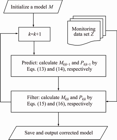
Fig. 1 Flowchart of dynamic imaging

In order to evaluate the dynamic imaging algorithm, a numerical dynamic model was built to produce synthetic data. The 2D model area with a background electrical conductivity 1×10^-3 S/m is divided to 30×30 grids, and the grid sizes are 0.1 m × 0.1 m. By following the time step, particles gathered at the center of the top section spread out as Eq. (2). The aim is to simulate the transportation of metallic contamination plume in an underground porous medium. In this numerical model, 3000 particles are employed. And the permeability, the porosity, the dynamic viscosity of solution and the fluid density are set to be 1×10^-11 m/s, 30%, 1×10^-3 Pa·s and 1×10³ kg/m³, respectively. Thus, according to Eq. (1), the Darcy velocity varies proportionally with the depth along y direction. With the model involved, the particles continue to diffuse and form a series of synthetic geoelectric section at different time step.

For convenience, the ratio of the electrical conductivity to the background, named the relative electrical conductivity, was used to describe the synthetic geoelectric sections. Figure 2 shows six relative electrical conductivity distribution snapshots of the particles diffusing process at time steps of 10, 30, 60, 100, 150 and 210, respectively.

The synthetic self-potential observation data can be obtained by forwarding these geoelectric model sections at different time steps. The finite element method was used to perform the forward and calculate the electric potential distribution. Then, the surface data points were selected with 5 cm interval to simulate a self-potential observation dataset. And a random noise of 30% of the self-potential values are added respectively to the synthetic data for each time step. These added noises are used to simulate the observation errors generated during the process of acquiring field data from a noisy measurement. Figure 3 shows the synthetic self-potential observation data at time steps of 10, 30, 60, 100, 150 and 210, respectively. The solid blue line is drawn from the directly forwarded data, and the red dashed line is drawn from the noise added data.

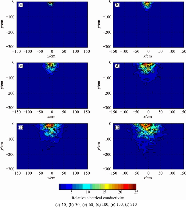
Fig. 2 Relative electrical conductivity distribution snapshots of 2D dynamic model at different time steps

By following the flowchart as Fig. 1, we input the noise added synthetic self-potential data into the extended Kalman filter recursion to perform the dynamic imaging. After alternately predicting and filtering, a series of resulting model sections were output.

As shown in Fig. 4, there are relative electrical conductivity distribution sections calculated from the corresponding synthetic self-potential observation data at time steps 10, 30, 60, 100, 150 and 210, respectively. Comparing Fig. 4 with Fig. 2, the dynamic imaging results match the original models very well. This demonstrates that the extended Kalman filter algorithm achieves dynamic imaging with high accuracy and a good performance on anti-noise.

3.2 Dynamic imaging using self-potential monitoring experiment data

A metallic ions diffusion monitoring experiment has been implemented in a sandbox in laboratory. Then, the laboratory measured time-lapse self-potential data were used to recover the diffusion process by the Kalman dynamic imaging. The sandbox is 1.0 m long, 0.5 m wide, and 0.5 m high. It was open at the top and filled with saturated fine sand with an average grain size of approximately 0.25 mm. And a small amount of KMnO₄ solution was uniformly mixed into the sand. A container filled with saturated FeCl₂ solution was set on top of a sandbox. The FeCl₂ solution can be dripped into the sand from the small opening hole on the bottom of the container. The leakage of the FeCl₂ into the sandbox will cause sand to change its electric conductivity due to the effects of the highly concentrated ferrous ions. Meanwhile, the ferrous ions react with KMnO₄ in the sandbox and induce redox reactions. The ionic reaction is as follows:

5Fe²⁺++8H⁺=Mn²⁺+5Fe³⁺+4H₂O         (19)

These redox reactions may induce self-potential anomalies that can be measured on the sand surface. As shown in Fig. 5, in order to measure the self-potential, a strip fixed with 18 lead wire non-polarized electrodes is placed on the top of the sandbox. Each electrode is 5 cm apart except electrodes 9 and 10 which is set to be 10 cm apart. Meanwhile, a reference electrode is set on the bottom of the sandbox. The self-potential differences between each of the measuring electrodes and the reference electrode are recorded by a multi-channel electric instrument. The instrument is named as WGMD-60 resistivity measurement system initially manufactured for resistivity, self-potential, and other geophysical exploration.

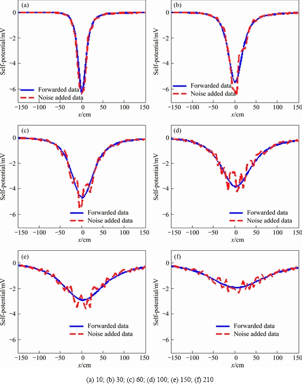
Fig. 3 Synthetic self-potential observation data at different time steps

Before the FeCl₂ solution starts to leak into the sandbox, the initial self-potential signals are measured at each electrode. All the measuring electrodes have potential values from -0.5 to 0.9 mV. The self-potential monitoring starts immediately after the FeCl₂ begins leaking. The self-potential data of each measuring electrode are recorded within a time interval of 30 s. All the measuring electrodes show some changes in their self-potential values while FeCl₂ solution is leaking into the sandbox. The multi-channel electric instrument shows a rapid down stroke of negative potential within the solution diffusion range. It also shows that the further the electrodes are away from the FeCl₂ diffusion center, the smaller the amplitude variation of self-potential signal is. Figure 6 shows the recorded monitoring self-potential curves at time from 30 to 240 s.

Fig. 4 Relative electrical conductivity distribution snapshots of reconstructed model by dynamic imaging at different time steps

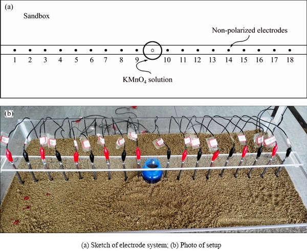
Fig. 5 Experimental setup

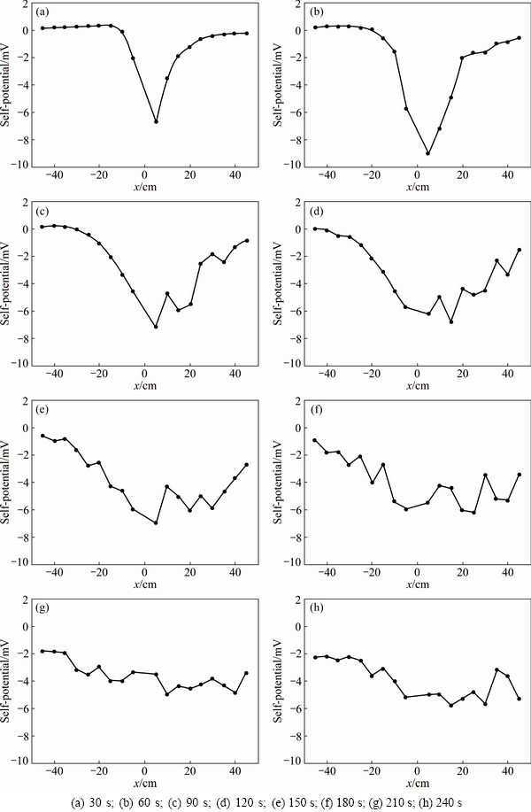
Fig. 6 Monitoring self-potential data recorded on electrodes in sandbox at different time

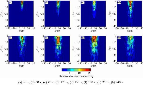
Fig. 7 Dynamic imaging of monitoring data at different time

Then, these monitoring self-potential data are processed by the Kalman dynamic imaging cycle. In a similar way to the synthetic case, the model state of the metallic ions diffusion evolves depending on the Darcy’s equation. Then, the Archie’s equation is used to transform the ionic concentration distribution to the electrical conductivity distribution. And the self-potential observation data were used to refine the electrical conductivity distribution. As the dynamic imaging results, a series of relative electrical conductivity distribution models were output. As shown in Fig. 7, these are imaging results at time from 30 to 240 s, respectively.

According to the results calculated from the Darcy’s model [21], the FeCl₂ plume reaches the bottom of the sandbox at time 180 s. The imaging results of self-potential monitoring data align well with the theoretical results. As shown in Fig. 7, the relative electrical conductivity distribution varies little after at time 180 s because the diffusion slowed down rapidly after the plume reaches the bottom. That means the dynamic imaging method is effective to invert the self-potential monitoring data and recover the dynamic process of metallic ions diffusion.

4 Conclusions

1) Based on the electrochemical properties of metallic ions, self-potential method was used to monitor the underground metallic contaminants. And a corresponding dynamic imaging method was proposed to interpret the monitoring self-potential data by using the extended Kalman filter.

2) Like other geophysical inversions, it is very difficult to recover a geoelectric model exactly only by a single self-potential observation. Thereby, instead of using regular inversion methods, the Kalman filter technique was used to perform dynamic imaging for the self-potential monitoring data. By combining the model evolving information with self-potential observation data to minimize possible inversion artifacts, the Kalman filter recursion can exactly recover the process of metallic ions diffusion in porous medium.

3) The noise added numerical test demonstrates that the dynamic imaging method can interpret self-potential monitoring data successfully. It also shows that the algorithm is effective, robust, and tolerance to noise.

4) The laboratory experiment proves that the metallic ions diffusion in porous medium can be monitored effectively by self-potential observation. Also, the laboratory monitoring data test proves that the dynamic imaging method can precisely retrieve the metallic ions plume even with being given very limited observation data at each time step. That is very meaningful to real metallic contamination monitoring.

Acknowledgments

We appreciate Miss Jian McKee for helping us improve the English expression. We also want to thank two anonymous reviewers and editors for their constructive comments and suggestions that greatly improved this manuscript.

References

[1] MAHAR A, WANG P, ALI A, ALI, A, AWASTHI M K, LAHORI A H, WANG Q, LI R H, ZHANG Z Q. Challenges and opportunities in the phytoremediation of heavy metals contaminated soils: A review [J]. Ecotoxicology and Environmental Safety, 2016, 126(4): 111-121.

[2] LIAO Ying-ping, WANG Zhen-xing, YANG Zhi-hui, CHAI Li-yuan, CHEN Jian-qun, YUAN Ping-fu. Migration and transfer of chromium in soil-vegetable system and associated health risks in vicinity of ferro-alloy manufactory [J]. Transactions of Nonferrous Metals Society of China, 2011, 21(11): 2520-2527.

[3] GALLAS J D F, TAIOLI F, FILHO W M. Induced polarization, resistivity, and self-potential: A case history of contamination evaluation due to landfill leakage [J]. Environmental Earth Sciences, 2011, 63(2): 251-261.

[4] PLACENCIA-GOMEZ E, PARVIAINEN A, HOKKANEN T, LOUKOLA-RUSKEENIEMI K. Integrated geophysical and geochemical study on AMD generation at the Haveri Au-Cu mine tailings, SW Finland [J]. Environmental Earth Science, 2010, 61: 1435-1447.

[5] RITTGERS J B, REVIL A, KARAOULIS M, MOONEY M A, SLATER L D, ATEKWANA E A. Self-potential signals generated by the corrosion of buried metallic objects with application to contaminant plumes [J]. Geophysics, 2013, 78(5): EN65-EN82.

[6] CASTERMANT J, MENDONCA C A, REVIL A, TROLARD F, BOURRIE G, LINDE N. Redox potential distribution inferred from self-potential measurements associated with the corrosion of a burden metallic body [J]. Geophysical Prospecting, 2008, 56(2): 269-282.

[7] REVIL A, TROLARD F, G, CASTERMANT J, JARDANI A, MENDOCA C A. Ionic contribution to the self-potential signals associated with a redox front [J]. Journal of Contaminant Hydrology, 2009, 109: 27-39.

[8] CUI Yi-an, ZHU Xiao-xiong, CHEN Zhi-xue, LIU Jia-wen, LIU Jian-xin. Performance evaluation for intelligent optimization algorithms in self-potential data inversion [J]. Journal of Central South University, 2016, 23(10): 2659-2668.

[9] DE CARLO L, PERRI M T, CAPUTO M C, DEIANA R, VURRO M, CASSIANI G. Characterization of a dismissed landfill via electrical resistivity tomography and  method [J]. Journal of Applied Geophysics, 2013, 98(11): 1-10.

[10] TOURLOS P, OGILVY R D, MELDRUM P I, WILLIAMS G. Time-lapse monitoring in single boreholes using electrical resistivity tomography [J]. Journal of Environmental and Engineering Geophysics, 2003, 8(1): 1-14.

[11] KIM J H, YI M J, PARK S G, KIM J G. 4-D inversion of DC resistivity monitoring data acquired over a dynamically changing earth model [J]. Journal of Applied Geophysics, 2009, 68(4): 522-532.

[12] KIM J H, SUPPER R, TSOURLOS P, YI, M J. Four-dimensional inversion of resistivity monitoring data through Lp norm minimizations [J]. Geophysical Journal International, 2013, 195(3): 1640-1656.

[13] OLDENBORGER G A , KNOLL M D, ROUTH P S, LABRECQUE D J. Time-lapse ERT monitoring of an injection withdrawal experiment in a shallow unconfined aquifer [J]. Geophysics, 2007, 72(4): F177-F187.

[14] MILLER C R, ROUTH P S, BROSTEN T R, MCNAMARA J P. Application of time-lapse ERT imaging to watershed characterization [J]. Geophysics, 2008, 73(3): G7-G17.

[15] ZHAO Yun-chao, GUI Xiao-chun, HONG Zhen-jie, LI Jian-yong. Kalman filter imaging of ionosphere TEC [J]. Chinese Journal of Geophysics, 2014, 57(11): 3617-3624. (in Chinese)

[16] ZHENG Wei, ZHANG Gui-bin. Application research on adaptive Kalman filtering for airborne gravity anomaly determination [J]. Chinese Journal of Geophysics, 2016, 59(4): 1275-1283. (in Chinese)

[17] ZHU Jian-jun, DING Xiao-li, CHEN Yong-qi. Dynamic model for land sliding monitoring under rigid body assumption [J]. Transactions of Nonferrous Metals Society of China, 2001, 11(2): 301-306.

[18] LEHIKOINEN A, FINSTERLE S, VOUTILAINEN A, KOWALSKY M B, KAIPIO J P. Dynamical inversion of geophysical ERT data: State estimation in the vadose zone [J]. Inverse Problems in Sciences and Engineering, 2009, 17(6): 715-736.

[19] LEHIKOINEN A, HUTTUNEN J M J, FINSTERLE S, KOWALSKY M B, KAIPIO J P. Dynamic inversion for hydrologic process monitoring with electrical resistance tomography under model uncertainties [J]. Water Resources Research, 2010, 46(4): 475-478.

[20] NENNA V, PIDLISECKY A, KNIGHT R. Application of an extended Kalman filter approach to inversion of time-lapse electrical resistivity imaging data for monitoring recharge [J]. Water Resources Research, 2011, 47(10): 599-609.

[21]  P, JARDANI A, REVIL A, HAAS A. Self-potential monitoring of a salt plume [J]. Geophysics, 2010, 75(4): WA17-WA25.

[22] REVIL A,  C A, ATEKWANA E A, KULESSA B, HUBBARD S S, BOHLEN K J. Understanding biogeobatteries: Where geophysics meets microbiology [J]. Journal of Geophysical Research, 2010, 115(G1): 379-384.

基于自然电场监测的金属污染物动态成像

崔益安^1,2,3，朱肖雄^1,2,3，魏文胜^1,2,3，柳建新^1,2,3，佟铁钢^1,2,3

1. 中南大学 地球科学与信息物理学院，长沙 410083；

2. 中南大学 有色资源与地质灾害探查湖南省重点实验室，长沙 410083；

3. 中南大学 教育部有色金属成矿预测重点实验室，长沙 410083

摘  要：提出了自然电场数据的动态成像方法。基于达西定律和阿尔奇公式，构建模拟孔隙介质中金属离子运动的动态模型。采用能斯特方程计算金属离子的氧化还原电位。在此基础上建立自然电场监测金属离子活动的状态模型和观测模型，利用扩展卡尔曼滤波技术对金属离子活动过程进行动态成像。模拟数据测试结果表明，该方法能有效将金属离子运动模型与自然电场观测数据融合，实现动态成像。进一步沙箱监测实验表明，自然电场法可以有效监测金属离子污染，利用动态成像方法可以有效重构金属离子的扩散过程。

关键词：动态成像；自然电场；金属污染；扩展卡尔曼滤波

(Edited by Xiang-qun LI)

Foundation item: Project (41574123) supported by the National Natural Science Foundation of China; Project (2013FY110800) supported by the National Basic Research Scientific Program of China

Corresponding author: Yi-an CUI; Tel: +86-731-88877075; E-mail: cuiyian@csu.edu.cn

DOI: 10.1016/S1003-6326(17)60205-X