J. Cent. South Univ. Technol. (2011) 18: 1614-1618

DOI: 10.1007/s11771-011-0880-6

Nonlinear correction of photoelectric displacement sensor based on least square support vector machine

GUO Jie-rong(郭杰荣)^{1, 2}, HE Yi-gang(何怡刚)², LIU Chang-qing(刘长青)¹

1. College of Physics and Electronics, Hunan University of Arts and Science, Changde 415000, China;

2. College of Electrical and Information Engineering, Hunan University, Changsha 410082, China

? Central South University Press and Springer-Verlag Berlin Heidelberg 2011

Abstract: A model of correcting the nonlinear error of photoelectric displacement sensor was established based on the least square support vector machine. The parameters of the correcting nonlinear model, such as penalty factor and kernel parameter, were optimized by chaos genetic algorithm. And the nonlinear correction of photoelectric displacement sensor based on least square support vector machine was applied. The application results reveal that error of photoelectric displacement sensor is less than 1.5%, which is rather satisfactory for nonlinear correction of photoelectric displacement sensor.

Key words: least square support vector machine; position; photoelectric displacement sensor; nonlinear correct

1 Introduction

Optical displacement sensor is widely used on the on-line measurement for boundary position in the industrial production and experiments such as steel rolling, textile and printing. It is also used to ensure the successful completion of tape, trimming border and overprinting pattern or to ensure a better damping effect and vibration isolation.

In theory, the relationship between input (displacement) and output (voltage) of the optical displacement sensor [1-3] is non-linear. The input (displacement)-output (voltage) data from optical measurement system must be corrected to improve the measurement accuracy. In the practical application, piecewise linear correction methods are commonly used. However, they are usually short of preciseness in some situations that require higher precision.

In order to improve the measurement accuracy of photoelectric sensors, researchers have made great efforts by various experimental and digital correction methods [4-11]. But, the phenomenon of inadequate precision still exists, which cannot meet the actual needs for testing high precision displacement parameters.

The support vector machine (SVM) is a new machine learning method [12-15], which is established on statistical learning theory, based on the structural risk minimization principle, and possesses good generalization ability.

The limited sample learning problem has shown a lot of performance better than the existing methods. As SVM algorithm is a convex quadratic optimization problem, it can guarantee to find the global optimal solution, and can solve the problem with the small sampling number, nonlinear relation and high dimension. Therefore, the least square support vector machine, (LS-SVM) [13], a nonlinear compensation method, is proposed, which can make optical displacement sensor linearized. The corrected network can be processed according to the linear characteristics, and the measurement accuracy is improved.

2 Nonlinear corrections of photoelectric displacement sensor based on LS-SVM

2.1 Principle of optical displacement sensor

Optical displacement sensor is a lateral semiconductor-based photo-detector device. It is a non-split-type photoelectric conversion device in a position to continuously detect the light point.

Practical optical displacement sensor generally uses the PIN structure, as shown in Fig.1. Its surface is P layer on light-sensitive side with output electrode on each side, the middle is I layer, and the bottom layer is highly doped N, to reverse bias voltage.

When the incident lights reach a point of the photosensitive surface of optical displacement sensor, photo-generated carriers are excitated after the photon absorption by semiconductor. Under transverse electric fields, carriers flow to both ends of the output electrode, forming the output current I₁ and I₂, and the ratio of I₁ to I₂ will change with the movement of light source position. The location of points of light could be determined according to the current signal proportion collected on electrodes.

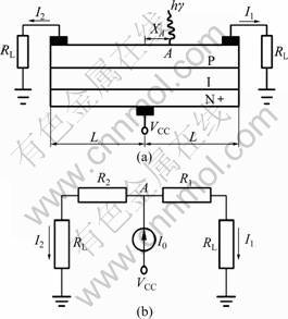
Fig.1 Measurement principle of photoelectric displacement sensor: (a) Structure; (b) Equivalent diagram

Suppose that light is at point A of photosensitive layer on optical displacement sensor, and the distance from the center is X_A. Let P layer resistance be uniform. The equivalent resistances from point A to the both sides of optical displacement sensor are R₁ and R₂, the load resistance is R_L, and R₁ and R₂ are far greater than R_L. The distance between the poles is 2L, the currents flowing through the poles are I₁ and I₂, and the total photocurrent is I₀. According to the Lucovsky equation of horizontal photoelectric effect, there is

I₀= I₁+ I₂                                                      (1)

where I₁=[(L-X_A)I₀]/(2L), and I₂=[(L+X_A)I₀]/(2L).

Therefore, it yields:

X_A =(I₂-I₁)L/(I₂+I₁)                                             (2)

If the currents I₁ and I₂ on the load resistance are measured, X_A can be calculated.

2.2 Calibration model of nonlinear optical displacement sensor

When the photoelectric displacement sensor is adopted in the displacement measurement, the output voltage signal goes through the transmitter, and the output can reflect the size of the displacement. Through the A/D, digital signals of the displacement can be obtained. Because there exists serious non-linearity between the output voltage and the measured displacement, it can be expressed as

    (3)

where y is the measured weight; U is output voltage of the optical displacement sensor; U_max is the maximum output voltage of optical displacement sensor; a₀, a₁, a₂ and a₃ are constant coefficients for the non-linear calibration. To eliminate the nonlinear error of optical displacement sensor, the output y of optical displacement sensor could be sent to a compensator whose characteristic function is z=F(y), where F(y)=f ^-1(y), and then the nonlinearity can be eliminated effectively.

Obviously, F(y) is a nonlinear function, and the output value z after compensation is the same as measured x, thus the optical displacement sensor has ideal characteristics. The process is shown in Fig.2.

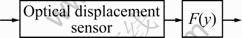
Fig.2 Sketch of non-linear correction process

In practice, the general nonlinear function F(y) cannot be accurately expressed. However, according to SVM theory, If k input samples, (y₁, z₁), (y₂, z₂), …,   (y_k, z_k), are known, a nonlinear projection can be found from the input space to the output space, which can project Y data in the highly dimensional feature space, and the linear regression of this space can carry through a certain linear function.

Noises existing in the optical displacement sensor (such as Gaussian noise) always affect the performance of system. The standard SVM algorithm has less resistance to the noise, and the computing speed is dependent on the number of sample data but not the dimension of input space. The larger the sample data, the more complex the corresponding quadratic programming problem to be solve, the slower the calculations and the longer the calculation time. The LS-SVM optimization index uses square item, and there are only equality constraints, but no inequality constraints, so the complexity of computation is simplified. Therefore, in this work, LS-SVM is used for the nonlinear calibration of optical displacement sensor.

LS-SVM selects a different loss function in the optimization objectives, which is distinguished from that in the standard SVM algorithm. The loss function uses the quadratic square of the error to replace insensitive loss function. Optimization is improved on the basis of the standard SVM:

                             (4)

s.t.  y_i= w^T?φ(x_i)+b+ε_i , ε_i >0，i=1，2，…，n

where ε_i is the slack variable; C is the penalty factor; b is the threshold value.

The corresponding Lagrange function is

  (i=1, 2, …, n) (5)

where c_i is the Lagrange coefficient.

Then, LS-SVM optimization problem is transformed into linear equation:

                                       (6)

where y=[y₁, y₂, …, y_n]^T；η_n is n-dimensional row vector; η_n=[1, 1, …, 1]；a=[a₁, a₂, …, a_n]^T, Ω_ij=φ(x_i) ?φ(x_j)=k(x_i, x_j), s is n-dimensional column vector; s=[1, 1, …, 1]^T; I is the identity matrix.

The nonlinear calibration model of optical displacement sensor is

                                         (7)

where x=[x₁, x₂, …, x_l], ,  and σ is kernel parameter.

2.3 Parameter optimization using chaos genetic algorithm

Penalty factor C and kernel parameter σ of calibration nonlinear model in optical displacement sensor can be optimized using chaotic genetic algorithm. Taking into account that the key of chaotic genetic algorithm is to determine the fitness function, the fitness function of this study is

                              (8)

where y_i is the desired output; f (x_i) is the actual output; e is a small positive number, and here it is10^-3.

An error function, MSE, is defined as a generalization performance evaluation indicator of nonlinear calibration model in optical displacement sensor:

                                         (9)

where M is the number of training samples of the optical displacement sensor. The optimization procedure for nonlinear calibration model parameters of optical displacement sensor using chaos genetic algorithm is as follows.

1) Coarse search

Step 1: Produce species chaos

The r-dimensional continuous space optimization problem can be expressed as

                                          (10)

s.t.   a_i≤X_i≤β₂, i=1, 2, …, r

where r is the number of optimization variables. Then, random numbers in (0,1), s₁, s₂, …, s_r, are generated as the initial values, which are put ??into an infinite number folding models s_n+1=4s_n(1-s_n) to produce r chaotic variables whose species size is N: (s₁¹, s₁², …, s₁^N)^T, (s₂¹, s₂², …, s₂^N)^T, …, (s_r¹, s_r², …, s_r^N)^T. The last value of each chaotic variable is saved into vector Z₀, Z₀=(z₁, z₂, …, z_r), where z₁=s₁^N, z₂=s₂^N, …, z_r=s_r^N, as the initial values for a fine search of the chaos variable.

Step 2: Coding

To avoid complex coding and decoding of binary, the real digital is used for encoding of each chromosome, that is, using r chaotic variables with species size of N to initialize the first chromosome. Taking the j-th chromosome for example, the initialization results can be expressed as

                                         (11)

Step 3: Solution space transformation

Each chromosome consisting of r chaotic variables with species size of N is protected from traversal space to the solution space of function optimization problem through the linear transformation. Therefore, the probability amplitude of each chromosome corresponds to a solution space optimization variable:

                           (12)

To ensure that the new range will not be out of the bounds, the following treatments are conducted: if X^j_i1i, then X^j_i1=a_i; if X^j_i2>b_i, then X^j_i2=b_i.

Step 4: Fitness calculation

Take the objective function shown in Eq.(10) as fitness function; use Eq.(8) to calculate the fitness of each chromosome and sort; record the best chromosome as P₀ and contemporary best chromosome as  If, then P₀=

Step 5: Conditions to determine cut-off algorithm

If P₀ remains constant after several generations of the coarse search, then the algorithm is ended, and the fine search phase begins. Save the current optimal solution X, otherwise the evolution of algebraic increase algorithm is conducted.

2) Fine search

Sequence Z_i is generated by the assignment phase of Z₀. Each element of the vector according to s_n+1=4s_n(1-s_n) continues to generate the chaotic sequence.

Step 1: Generate search variables

                                      (13)

where η_i is a constant for the adaptive adjustment, and it can be adaptively determined by Eq.(14):

                                             (14)

where K₂ is the number of fine iterations.

Clearly, as K₂ increases, η_i will gradually decrease. The main reason is that the large change of (s₁, s₂, …, s_n) in the early fine iterative search needs a larger adaptive constant η_i. As K₂ increases, the solution gradually approaches the advantages, so that a smaller η_i is needed in fine search within the small scope in

Step 2: Evaluation of X_i^* with objective function

Calculate the corresponding f(X_i^*); if f(X_i^*)>f(X), then f(X)=f(X_i^*), otherwise abandon X_i^*.

Step 3: If it meets the cut-off criterion E<10^-5, then the searching is stopped, and the optimal solution X is the output, otherwise go to fine search stage Step 1.

3 Application of photoelectric displacement sensor nonlinear calibration based on LS- SVM

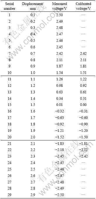
After accurate measurement of the actual displacement by micrometer screw and the output voltage, data of optical displacement sensors to be calibrated are obtained, as listed in Table 1.

Through observation, a good linear relationship happens within the displacement range of 0.7-2.3 mm. Select this section to fit. Therefore, take 7-27 calibration voltage data of the optical displacement sensor as the nonlinear calibration input data; find the relationship between displacement and voltage. Using methods of SVM with linear kernel method and LS-SVM for training support vector machines for non-linear calibration, the relationship between corrected displacement and voltage of optical displacement sensor is shown in Table 1. Based on the nonlinear calibration using LS-SVM of optical displacement sensor, the resulting relationship equation in the linear range between displacement and voltage is

U=4.97-3.22y                                              (14)

The fitting linearity of optical displacement sensors is 0.998 7, and the maximum error is less than 1.5%, indicating that the improved high-precision optical sensor can meet the requirements.

The convergence rate about the non-linear errors of photoelectric displacement sensor is shown in Fig.3. It can be seen that the use of LS-SVM method can greatly reduce the training times.

Table 1 Standardization data of photoelectric displacement sensor

By comparing the measured displacement values obtained by screw micrometer with those ??obtained by nonlinear calibration correction LS-SVM-based and SVM-based photoelectric displacement sensors, the relative error curve of displacement values are shown in Fig.4.

Figure 4 shows that the absolute value of relative error of displacement of ??optical displacement sensor obtained by LS-SVM nonlinear correction is less than 1.5%. If the sample size increases, more experimental data for training are used, and the measurement accuracy can be further improved. The absolute values of relative error of displacement of ??optical displacement sensor obtained by LS-SVM nonlinear calibration should be -3.9%-4.0%. Therefore, using LS-SVM corrected optical displacement sensor can attain high accuracy, which can fully meet the requirements of industrial production, such as rolling mill, textile, printing, vibration isolation and other experimental displacement real-time online measurement.

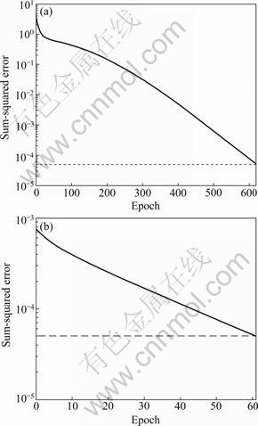
Fig.3 Convergence rates about non-linear errors of photo- electric displacement sensor: (a) SVM method; (b) LS-SVM method

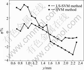
Fig.4 Relative errors of position value about photoelectric displacement sensor after nonlinear correction

4 Conclusions

1) The nonlinear correction model based on LS-SVM method is established. By using chaos genetic algorithm, the penalty factor and kernel parameter of LS-SVM are optimized. The application examples show that the accuracy can be achieved at 1.5%, which can meet the needs for most applications.

2) LS-SVM based method for the photoelectric displacement sensor nonlinear correction is simple and fast. The actual amount of calculation is very small. It has a strong ability to curve fitting and can be widely used in roughness and roundness precision testing conditions.

References

[1] XU Jun, PENG Dong-lin, WAN Wen-lue, YANG Wei. New way of producing electrical traveling wave signal based on photoelectricity technology in design of time-grating displacement sensor [J]. Chinese Journal of Sensors and Actuators, 2007, 20(3): 532-535. (in Chinese)

[2] XU Tao, Lu Hai-bao, LUO Wu-sheng. A robust photoelectric angular position sensor especially for a steerable underground boring tool original [J]. Sensors and Actuators A: Physical, 2005, 120(2): 311- 316.

[3] YU Yuan, DING Mei-ying, ZHANG Lian-kai. The algorithmic analysis of linear approximation for characteristic region of displacement sensor [J]. Chinese Journal of Sensors and Actuators, 2010, 23(6): 840-843. (in Chinese)

[4] SHI Ze-lin, KANG Jiao, SUN Rui. BP NN-based method for lens distortion correction of large-field imaging [J]. Opt Precision Eng, 2005, 13(3): 348-353. (in Chinese)

[5] LING Wei, WANG Zhi-qian, GAO Feng-duan. Real time digital correction for distortion in photoelectronic measuring system [J]. Opt Precision Eng, 2007, 15(2): 277-282. (in Chinese)

[6] QIAO Yan-feng, GAO Feng-duan, WANG Zhi-qian, ZHAO Yan, LI Jian-rong. Distortion correction for the photoelectricity measuring system based on the cubic fitting equation[ J]. Opto-Electronic Engineering, 2008, 35(6): 28-31. (in Chinese)

[7] YU Dong-bao, SU Zhen-wei, YAN Kai-hua. A new type of machine vision systems with algorithm for image correction [J]. Laser & Infrared, 2008, 38(11): 1173-1176. (in Chinese)

[8] BAI Xu-guang, CAI Sheng, GAO Feng-duan, QIAO Yan-feng, DAI Ming. Distortion correction for photoelectric measuring system based on BP neural network [J]. Laser & Infrared, 2010, 40(1): 79-82. (in Chinese)

[9] CAI S H, LIQ A, QIAO Y F. Camera calibration of attitude measurement system based on BP neural network [J]. Journal of Opoelectronics Laser, 2007, 18(7): 832-834. (in Chinese)

[10] WANG Zi-qiang, LI Yin-mei, LOU Li-ren, WEI Heng-hua, WANG Zhong. Application of BP neural network to nonlinearity correction of optical tweezer force [J]. Opt Precision Eng, 2008, 16(1): 6-10. (in Chinese)

[11] ZHENG Feng-xun, JI Shi-peng. An improved nonuniformity correction algorithm for irfpa based on neural network [J]. Laser & Infrared, 2008, 38(9): 937-938. (in Chinese)

[12] VAPNIK V. Statistical learning theory [M]. New York: Wiley, 1998: 12-35.

[13] E Jia-qiang. Intelligent fault diagnosis and its application [M]. Changsha: Hunan University Press, 2006: 70-130. (in Chinese)

[14] ANTHONY T C, GOH S H. Support vector machines: Their use in geotechnical engineering as illustrated using seismic liquefaction data [J]. Computers and Geotechnics, 2007, 34(5): 410-421.

[15] JIANG X F, YI Z, L? J C. Fuzzy SVM with a new fuzzy membership function [J]. Neural Computing and Application, 2006, 15(2): 268-276.

(Edited by YANG Bing)

Foundation item: Project(50925727) supported by the National Fund for Distinguish Young Scholars of China, Project(60876022) supported by the National Natural Science Foundation of China, Project(2010FJ4141) supported by Hunan Provincial Science and Technology Foundation, China; Project supported by the Fund of the Key Construction Academic Subject (Optics) of Hunan Province, China

Received date: 2011-03-04; Accepted date: 2011-07-11

Corresponding author: GUO Jie-rong, Associate Professor, PhD; Tel: +86-736-7186121; E-mail: jierong_guo@yahoo.com.cn