J. Cent. South Univ. Technol. (2011) 18: 1184-1192

DOI: 10.1007/s11771-011-0821-4

Forecasting model of residential load based on general regression neural network and PSO-Bayes least squares support vector machine

HE Yong-xiu(何永秀), HE Hai-ying(何海英), WANG Yue-jin(王跃锦), LUO Tao(罗涛)

School of Economics and Management, North China Electric Power University, Beijing 102206, China

? Central South University Press and Springer-Verlag Berlin Heidelberg 2011

Abstract: Firstly, general regression neural network (GRNN) was used for variable selection of key influencing factors of residential load (RL) forecasting. Secondly, the key influencing factors chosen by GRNN were used as the input and output terminals of urban and rural RL for simulating and learning. In addition, the suitable parameters of final model were obtained through applying the evidence theory to combine the optimization results which were calculated with the PSO method and the Bayes theory. Then, the model of PSO-Bayes least squares support vector machine (PSO-Bayes-LS-SVM) was established. A case study was then provided for the learning and testing. The empirical analysis results show that the mean square errors of urban and rural RL forecast are 0.02% and 0.04%, respectively. At last, taking a specific province RL in China as an example, the forecast results of RL from 2011 to 2015 were obtained.

Key words: residential load; load forecasting; general regression neural network (GRNN); evidence theory; PSO-Bayes least squares support vector machine

1 Introduction

With the rapid development of the economy and the adjustment of economic structure in China, the proportion of residential load (RL) is increasing gradually and will continue to increase. RL is  influenced by residential living standard, living habit, geographical environment and so on. Forecasting RL scientifically and reasonably can make appropriate decisions for power planning and demand-side management.

The theoretical study of influencing factors and methods of RL started early. Influencing factors include alternative energy, family member, appliances, temperature, holidays, seasons and salary, etc.

At present, the common forecast methods include the per capita RL method, which fails to ensure scientific forecast results, the method based on the classification of terminal electricity consumption, which fails to collect the statistical data [1], and the multiple regression method [2-5], which cannot fully obtain the data about RL and influencing factors. In addition, the economic data are subjected to certain macro-control policy influences. So, the regression results reflect the economic law less. Other forecast methods include the polynomial regression model [6], the error correction model [7], the dynamic analysis model [8], the adaptive neural fuzzy inference system [9], the pseudo-panel data model [10], and so on. The methods above also have difficulties in collecting statistic data, so the applicability and accuracy of RL forecasting in China need to be further studied. Reference [11] applied a neural network to load forecasting in the circumstance of the competitive market. The related assumptions about input variables are simple, but the training parameters and numbers of layers and nodes need to be set artificially. So, the forecast accuracy needs to be further improved, and the problem of a local optimum exists in the process of training. In Ref.[12], a SVM with immune algorithm (IA) was presented to forecast the electric loads, where IA was applied to the parameter determination of SVM. The empirical results indicated that it resulted in better forecasting performance than the other methods, namely SVMG, regression model, and ANN model. A combined model of self-adaptive partical swarm optimization (APSO) and support vector machine (SVM) was put forward in Ref.[13]. APSO was applied to make the parameter determination of SVM better. In Ref.[14], a multi- layered perception neural network model was proposed; however, it needed too much information and time. In Ref.[15] a hybrid intelligent system was presented combining the wavelet kernel support vector machine and particle swarm optimization for demand forecasting and it was proved that this method was better than other traditional methods. Then, a new load forecasting model was presented based on hybrid particle swarm optimization with Gaussian and adaptive mutation (HAGPSO) and wavelet v-support vector machine (Wv-SVM) [16]. The methods of SVM and PSO were used in Ref.[17] in forecasting short-term price in electricity market. NIU et al [18] combined the ant colony optimization with SVM and achieved greater forecasting accuracy. However, the research above has not put forward a systemic and scientific RL forecast model, and influencing factors selection of RL has not been fully considered. In addition, the intelligent models have limitations in choosing parameters.

In the Bayes method, the uncertainty of all forms is expressed with the probability method, the process of learning and reasoning is realized through probability rules, and the analysis results are expressed as the probability distribution of random variables. As a new bionic evolutionary algorithm, the PSO method works based on the swarm and the fitness. The best location of particles can be recorded, and the information is shared between particles. The complex processes of selection, cross, and variation do not exist. In addition, it has the advantages of global optimization, fast convergence, and so on. In this work, the evidence theory is applied to combine the methods above. Then, suitable parameters of the LS-SVM model are determined. In addition, a general regression neural network (GRNN) is used to sort the degree of influencing factors, and the degree of factors at high level are selected as input variables. One smoothness factor needs to be adjusted in GRNN, which belongs to the radical basis function neural network (RBF). The learning process is fully dependent on samples, so the influence of subjective factors can be avoided to the maximum extent.

2.2 Key factors selection based on GRNN

RL is influenced by many factors, including economic factors, such as salary, power price, alternative energy price, housing condition and possession quantity of household appliance, and non-economic factors, such as population, living habits, urbanization rate and  climate, as shown in Fig.1. Furthermore, residential load is also influenced by demand-side management measures, power price control, reconstruction of distribution network, promotion of RL, competition in the energy market, national policy of energy conservation, and so on.

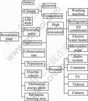
Fig.1 Residential load influencing factors

General regression neural network (GRNN) was originally proposed in 1991 [19-20]. The GRNN is one of the radial basis function neural networks, which is based on non-linear regression theory. It regards sample data as a posteriori condition, and the Parzen nonparametric estimation is carried out. Then, according to the rule of the maximum probability, the network output is calculated. It can approach a discontinuous function at any accuracy. The network converges to the optimized regression surface, which is accumulated on the most samples. And the learning rate is fast. It also has better learning performance. In addition, irregular data can be used in the network.

The GRNN consists of four layers: input layer, pattern layer, summation layer and output layer, as shown in Fig.2. X=[x₁, x₂, …, x_m]^T is the input vector, and Y=[y₁, y₂, …, y_l]^T is the output vector.

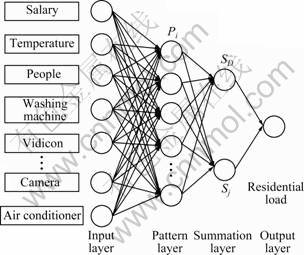
Fig.2 GRNN topology of selecting factors of RL forecast

Based on GRNN, the steps of selecting the   factors of RL forecasting are described as follows.

It is assumed that the joint probability density function of variables x and y is f(x, y). X is the observed value of x. So, relative to x, the regression of y can be expressed as

                         (1)

The unknown probability density function f(x, y) can be obtained through the observed value of x and y, and the nonparametric estimation can be expressed as

(2)

where X_i and Y_i are the observed values of random variables x and y, respectively; n is the number of samples; m is the dimensions of random variable x and f(x, y) is replaced by

Based on Eq.(1), the estimation value  is obtained by exchanging the sequence of integration and summation:

 (3)

where  is the weighted mean of whole samples. The weight of observed value Y_i is the exponent of the squared Euclid distance between corresponding samples X_i and X.

Step 1: The annual sample is set as input data. The number of input neurons is equal to the number of factors influencing RL forecasting, and each neuron presents data to the second layer directly, namely, the pattern layer.

Step 2: The number of pattern neurons is equal to the number of cases in the training set n. A typical pattern neuron i attains the data from the input neurons and computes an output P_i using the transfer function:

           (4)

where σ is the smoothing parameter, and P_i is the weight of observed value Y_i.

Step 3: The summation neurons include two kinds of neurons. One is simple arithmetic summation, which sums the outputs of pattern neurons. The weight between the pattern neurons and the summation is set at 1, and the transfer function S_D can be expressed as

                                                    (5)

The other is weighted summation. The weight between the neuron i of pattern neurons and the neuron j of summation neurons is the element j of output sample Y_i. The transfer function of summation neurons can be expressed as

                                 (6)

Step 4: The number of output neurons is equal to the dimension of output vector, l. Then, output neuron performs the following division to obtain the GRNN regression output y_j:

                                   (7)

Step 5: The testing samples are chosen by extracting some continuous samples randomly from training samples. It is assumed that the smoothness factor is increased by ?σ and the range is [σ_min, σ_max]. In the learning sample, the other samples are used for training except one sample. The error between estimation value and actual value is obtained. The process is repeated until each sample is excluded once, and the error series could be obtained. The MSE (mean square error, E) is applied to evaluate the network performance and expressed as Eq.(8). The optimized smoothness factor which has the minimum error is used for the final network training:

                                        (8)

The factor weight P_i influencing RL forecasting is determined while the smoothness factor is optimized. If P_i meets the constraint of Eq.(9), the factor i can be chosen as one of the final influencing factors, which is used for RL forecasting:

                                        (9)

3.3 RL forecasting model based on PSO- Bayes-LS-SVM

3.1 Bayes-LS_SVM regression algorithm

Give a set of training data {(x_i, y_i)|i=1, 2, …, n}, whereis the input of training set whose dimension is d and it is also the number of influencing factors of RL forecasting;is the output of training set. The dimension of RL forecasting model is one, namely, RL. Non-line mapping can be adopted as

                           (10)

To map original input space to higher dimensional feature space, an optimum decision function can be constructed as

                                      (11)

where w=(w₁, w₂, …, w_k), is a vector of weights in the high dimensional feature space; b is a constant, bR. By the structure risk principle, the following optimization problem can be obtained:

                                  (12)

where ||w||² is the regularization term, i.e. confidence interval, which controls the complexity of model; c is a regularization parameter; R_emp is the error term, i.e. empirical risk in learning theory. In the standard SVM model, the one degree term of error ξ_i is used as the loss function in the optimization. However, the quadratic term of error ξ_i is used in the LS-SVM model, whose constraints are equal. The optimization problem of the LS_SVM regression can be formulated as

                                     (13)

The Lagrangian approach is used to optimize the problem and Eq.(14) can be acquired:

(14)

whereis defined as kernels function of symmetric function which is based on the Mercer’s condition. Finally, a_i and b can be obtained by LS, and the nonlinear forecast function is obtained as

                                     (15)

3.2 Parameters optimization based on Bayesian

The Bayesian evidence framework divides the inference into three distinct levels. The Bayesian evidence framework is applied to the LS_SVM regression algorithm in order to select optimal regularization and optimal kernel parameters, w and b. Training of the SVM regression can be statistically interpreted in Norm 1 inference. The optimal regularization parameter c can be inferred in Norm 2 inference. The optimal kernel parameter selection σ in the SVM regression can be inferred in Norm 3 inference. The basic idea of model selection within the Bayesian evidence framework is to maximize the posterior probability of parameter distribution to obtain the optimal parameter [21].

1) Norm 1 inference

To be convenient, optimization objective is divided by c and then 1/c is replaced by λ. For a given model H with parameter vector of k dimensions, distribution p(D|w, b, λ, H) exists in the dataset D, where p(w, b|λ, H) is the prior probability. The optimum value of w and b can be determined by the posterior of the maximum parameters. The posterior of w and b is

                            (16)

2) Norm 2 inference

Regularization parameter λ of LS-SVM is referred by the Bayesian rule. The greatest possible value of λ can be determined by maximizing the posterior probability of λ as p(λ|D, σ). The posterior probability of λ can be obtained as

      (17)

3) Norm 3 inference

The optimal value of kernel parameter σ of LS-SVM can be obtained by examining their posterior probabilities:

                                     (18)

Then, the optimal kernel parameter value is σ_j corresponding to the maximum value of the radial basic function (RBF) kernel function.

3.3 Parameters optimization based on PSO

The PSO method is one of the optimized tools based on iteration. Random solutions are initialized at first. Then, the optimized value is found through continuous iteration. When the PSO method is used for finding the optimized parameters of LS-SVM, λ and σ, it is assumed that the number of particles is n, and each particle is expressed as a vector x_i=(x_i1, x_i2)^T, which represent λ and σ, respectively, and the number of dimensions is two. The fitness of particle x_i=(x_i1, x_i2)^T is the error value, which is obtained from the forecasting process by applying the LS-SVM model. At the beginning of optimization, random solutions are initialized, and then each particle performs iteration continuously until the terminal condition is met. In addition, the particle which has the minimum error is the optimized solution:

 (19)

                                                   (20)

(i=1, 2, …, n; j=1, 2, …, m)

where the number of particles is n; the number of dimensions is two; v^k is the offset and x^k is the location of the particle when the iteration number is k; c₁ and c₂ are the positive constants; r₁ and r_i are the random numbers which belong to [0, 1]; w_i is the coefficient of momentum term; p_best is the minimum error of each particle; g_best is the minimum error of iteration.

The process of the PSO method applied in this paper is shown in Fig.3.

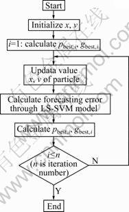
Fig.3 Optimization process of parameters in SVM based on PSO

In the process of the LS-SVM model, the form of original input space to higher dimensional feature space is determined by the type and the parameter of kernel function. The training error and the degree of complexity of the model are controlled by the regularization parameter c. So, it is necessary to adjust the parameters in order to obtain better performance.

The problem of choosing optimized parameters is turned into finding the optimized particle in a given space which has the minimum error.

3.4 RL forecasting model based on GRNN and PSO- Bayes-LS-SVM

The step of RL forecasting model based on GRNN and PSO-Bayes-LS-SVM is shown in Fig.4.

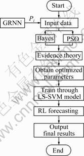
Fig.4 Process of RL forecasting model based on GRNN and PSO-Bayes-LS-SVM

The steps of RL forecasting model based on GRNN and PSO-Bayes-LS-SVM are described as follows.

Step 1: Establish regression function

The key factors of RL based on GRNN are the inputs of SVM, and RL is the output. According to Eq.(10), the optimal regression function is described as Eq.(11).

Step 2: Determine kernel function and parameters

The RBF kernel is adopted, and the regularization parameter and kernel parameter are determined by the methods of Bayes and PSO, respectively. The weights of parameters are determined by the evidence theory. And then, through weighted summation, the final regularization parameter λ and kernel parameter σ can be obtained. The optimization utility is obtained from the fuzzy utility set, namely, H={H₁, H₂, H₃, H₄, H₅}= {higher, high, common, low, lower}={1 0.8, 0.5, 0.3, 0.1}. The optimization utility of the above methods is evaluated by some experts. Based on the evidence theory, the evaluation of each expert is combined through Dempster rules. Then, the final values  and  could be obtained. Considering the fuzzy utility set, the utility values of the above methods, u_Bayes and u_PSO, can be calculated:

                                          (21)

                                            (22)

Based on the utility values of the above methods, the weighs of Bayes and PSO, ω_Bayes and ω_PSO, can be obtained:

                                     (23)

                                             (24)

Then, the final parameters can be obtained as

                               (25)

                         (26)

where λ_Bayes and λ_PSO are the regularization parameters determined by the methods of Bayes and PSO, respectively, and σ_Bayes and σ_PSO are the kernel parameter determined by the methods of Bayes and PSO, respectively.

Step 3: Establish forecasting model of residential load.

The optimization problem and constraints are established as Eq.(13), and optimization regression function coefficient is obtained by the Lagrangian approach. The forecasting model of RL is then established as Eq.(15).

Step 4: Forecast RL

The forecasting model of future RL can be obtained through inputting the important influencing factors of RL and imitation learning.

4.4 Case study

4.1 Data sources

Data in this work come from Statistical Yearbook [22] of specific province in China. The 15 input variables are selected in 1995-2008, including salary, population, temperature, per capita housing area, electric variables number and appliances, such as refrigerator, washing machine, air conditioner, TV, home computer, camera, music centre, microwave oven, electric water heater and vidicon. The output variable is residential load of the specific province during 2000-2008.

4.2 Key factors selection based on GRNN

Based on the Matlab7.0 platform and training analysis of GRNN, the errors at different smoothness values are calculated. By comparing the errors and the weights obtained from GRNN, the factors which influence the error of training results much are chosen as the final input variables. The input variables of urban areas include salary, population, temperature, per capita housing area, TV, refrigerator, washing machine, air conditioner and home computer. The input variables of rural areas include population, temperature, salary, per capita housing area, TV, washing machine, air conditioner and electric water heater. In this work, the data from 2000 to 2008 are chosen as training samples, and four continuous samples out of nine are chosen as the testing set. The smoothing parameter σ=0.1, 0.2, 0.3, 0.4, and the errors between actual values and forecasting values are shown in Fig.5. It is concluded that the least errors appear when σ=0.1.

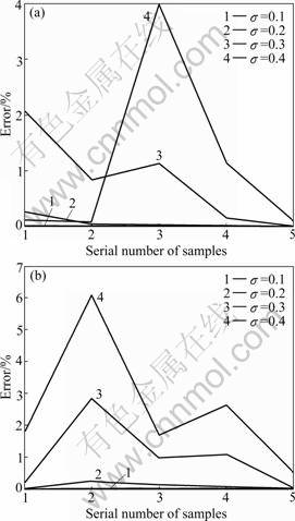
Fig.5 Effects of different smoothness values on error: (a) Urban; (b) Rural

4.3 Data pretreatment and parameters determination

Extremum method is used for standardized processing of input and output variables:

                                                (27)

where x_ij is the initial data; m_j is the minimum; M_j is the maximum;  is non-dimensional value, and [0,1].

Though standardized processing using Eq.(27), input and output variables are translated into the numbers between 0.1 and 0.9. (The input variables are the factors chosen by GRNN, and the output variables are the urban (rural) RL).

The regularization parameter λ and the kernel parameter σ are determined as follows.

Step 1: The process of parameters optimization is realized using the calculation software toolbox LS_SVMlab1.5. In the urban RL, λ is 10 879 and σ is 57.62. In the rural RL, λ is 740.74 and σ is 1 337.3.

Step 2: The process of parameters optimization is realized through PSO. It is assumed that the numbers of particles and iterations are 30 and 200, respectively. The error of iteration is calculated by the fitness function. The fitness values of each generation relative to urban RL and rural RL are shown in Fig.6.

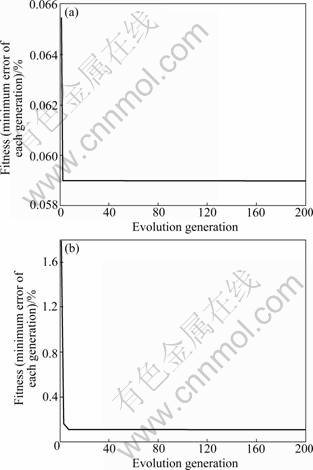
Fig.6 Fitness curves of RL forecasting: (a) Urban; (b) Rural

In the circumstance of the minimum error, in the urban RL, λ is 2 000 and σ is 20; in the rural RL, λ is    1 997.1 and σ is 20.

Step 3: Based on the evidence theory, the weights of parameters are determined. Then, the final λ and σ can be obtained. The weights of Bayes and PSO are 0.46 and 0.54, respectively. Now, the final parameters can be obtained. In the urban RL, λ is 6 024.34; in the rural RL, λ is 1 359.261. Through continuous testing, when σ is 20, the forecasting effect is better.

4.4 Forecasting results

4.4.1 Forecasting error test

Because of the limitation of data resource, the data in 1995-2008 are trained and tested. The forecasting errors are calculated as Eq.(28), and mean square error (MSE, E) is chosen for evaluating the forecasting errors as Eq.(29):

 (i=0, 1, 2, …)                         (28)

 (n=0, 1, 2, …)                       (29)

where ε_i is error; x_i is the true value;  is the corresponding forecast value; E is MSE;  is the average value of errors.

The comparisons between actual and predictive values of urban and rural RL forecasting results in 2002- 2008 are listed in Table 1 and Table 2, respectively.

Table 1 Comparison between actual and predictive values of urban RL forecasting results in 2002-2008 (GW?h)

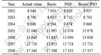
Table 2 Comparison between actual and predictive value of rural RL forecasting results in 2002-2008 (GW?h)

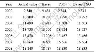
The forecasting errors of urban and rural RL using different methods are shown in Fig.7, the forecasting error of the PSO method is less than that of the Bayes method. The forecasting error of combined method above is less.

4.4.2 Comparison forecasting errors

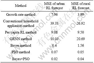
In order to prove the validity of the model, mean square error (MSE) is used to conduct the error evaluation as Eq.(29), and the evaluation results are compared with forecast errors of other methods. Finally, the forecast errors of various methods are listed in Table 3.

The prediction model of conventional household appliances can be described as

                                                (30)

where b_i=P_i×h_i, c=p/d. y is the residents consumption, n is the number of species of household appliances, i is the i-th class household appliance, a_i is the number of the i-th class household appliance ownership, b_i is the unit consumption of the i-th class household appliance, P_i is the power of the i-th class household appliance, h_i is the time used of the i-th class household appliance in a year, c is the number of households, P is the population in the predicted year, and d is the average size of every household.

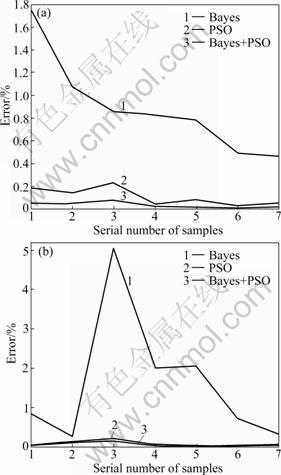
Fig.7 Forecasting errors of RL under different methods:     (a) Urban; (b) Rural

Table 3 Error comparison of RL forecasting (%)

The prediction model of growth rate can be described as

 (n=0, 1, 2, …)                              (31)

where v is the growth rate of RL; a₀ is RL in the based period; a_n is RL after n years.

Then, the future RL can be forecasted through translating Eq.(31) into Eq.(32):

 (n=0, 1, 2, …)                                 (32)

In the prediction model of per capita RL, per capita RL can be obtained through Eq.(31) and Eq.(32). Then, RL can be described as

 (n=0, 1, 2, …)                                (33)

where  is per capita RL; p_n is people number; a_n is RL.

As shown in Table 3, the MSE values of urban RL of growth rate method, conventional household appliances method, per capita RL method and GRNN method are 7.96%, 39.33%, 9.08%, 10.03%, respectively. The forecast error of the model proposed in this work is 0.02%, far lower than other methods. So, the combined model of GRNN and LS-SVM is the most accurate forecasting method in the above four methods. In this work, before forecasting RL with LS-SVM, GRNN model is used to select key factors of RL as the input and output variables. And then, the optimization results of the Bayes and the PSO are combined through the evidence theory. It considerably induces the errors. Among the above forecasting methods, there are not only conventional forecasting methods such as growth rate method, and conventional household appliances method, but also neural network method such as GRNN method. Through the comparison with conventional forecasting methods, it is concluded that the combined model performs more accurately. And through the comparison with the neural network method, whose basic data are the same as those in the combined model, the error from the basic data is excluded. Therefore, the combined model of GRNN and PSO-Bayes-LS-SVM can overcome the above shortcomings and minimize errors.

4.4.3 RL forecasting results

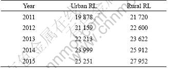
The forecasting results of RL of specific province in China based on the model proposed in this work are listed in Table 4.

Table 4 Forecasting results (GW?h)

5 Conclusions

1) Through analysis of the RL influencing factors with GRNN, it is concluded that the accuracy of the forecasting model will be improved if the key influencing factors are determined scientifically.

2) The critical step of applying LS-SVM is how to determine the optimized parameters. The Bayes method is dependent on probability rules, and the basis of the PSO method is finding the optimized solutions in a given space. The above methods are combined by the evidence theory, and the optimized parameters are obtained. Based on the empirical calculation, the forecasting errors of urban and rural RL are 0.02% and 0.04%, respectively. It is significantly better than single forecasting method.

3) It is found that the urban and rural RL are     25 251 and 27 952 GW?h in 2015, respectively, in specific province of China through applying the model proposed.

References

[1] SONG K B, HA S K. Hybrid load forecasting method with analysis of temperature sensitivities [J]. Transactions on Power Systems, 2006, 21(2): 869-877.

[2] LUTZENHISER L. Social and behavioral aspects of energy use [J]. Annual Review of Energy and the Environment, 1993, 18: 247-289.

[3] SONG K B, BAEKY S, HONG D H, Jang G. Short-term load forecasting for the holidays using fuzzy linear regression method [J]. Transactions on Power Systems, 2005, 20(1): 96-102.

[4] CHO M Y, HWANG J C, CHEN C S. Customer short term load forecasting by using ARIMA transfer function model [C]// EMPD International Conference on Energy Management and Power Deliver. Singapore, 1995: 317-322.

[5] BECCALI M, CELLURA M, BRANO V L, MARVUGLIA A. Short-term prediction of household electricity consumption: Assessing weather sensitivity in a Mediterranean area [J]. Renewable and Sustainable Energy Reviews, 2008, 12(8): 2040-2065.

[6] BOUKARY O. Household energy preferences for cooking in urban Ouagadougou Burkina Faso [J]. Energy Policy, 2006, 34(18): 3787- 3795.

[7] HOLTEDAHL P, JOUTZ F L. Residential electricity demands in Taiwan [J]. Energy Economics, 2004, 26(2): 201-224.

[8] HALVORSEN B. LARSEN B M. The flexibility of household electricity demand over time [J]. Resource and Energy Economics, 2001, 23(1): 1-18.

[9] YING Li-Chih, PAN Mei-chiu. Using adaptive network based fuzzy inference system to forecast regional electricity load [J]. Energy Conversion and Management, 2008, 49(2): 205-211.

[10] BERNARD J T, BOLDUC D, YAMEOGO N D. A pseudo-panel data model of household electricity demand [J]. Resource and Energy Economics, 2011, 33(1): 315-325.

[11] MANDAL P, SENJYU T, FUNABASHI T. Neural networks approach to forecast several hour ahead electricity prices and loads in deregulated market [J]. Energy Conversion and Management, 2006, 47(15/16): 2128-2142.

[12] HONG Wei-chiang, Electric load forecasting by support vector model [J]. Applied Mathematical Modeling, 2009, 33(5): 2444-2454.

[13] HUANG Yue, LI Dan, GAO Li-qun, WANG Hong-yuan. A short-term load forecasting approach based on support vector machine with adaptive particle swarm optimization algorithm [C]// Chinese Control and Decision Conference. Guilin, China, 2009: 1448-1453.

[14] MIRHOSSEINI M, MARZBAND M, OLOOMI M. Short term load forecasting by using neural network structure [C]// ECTI-CON International Conference. Chonburi, Thailand, 2009: 240-243.

[15] WU Qi. Product demand forecasts using wavelet kernel support vector machine and particle swarm optimization in manufacture system [J]. Journal of Computational and Applied Mathematics, 2010, 233(10): 2481-2491.

[16] WU Qi. Power load forecasts based on hybrid PSO with Gaussian and adaptive mutation and Wv-SVM [J]. Expert Systems with Applications, 2010, 37(1): 194-201.

[17] GAO Ci-wei, BOMPARD E, NAPOLI R, CHENG Hao-zhong. Price forecast in the competitive electricity market by support vector machine [J]. Physica A: Statistical Mechanics and its Applications, 2007, 382(1): 98-113.

[18] NIU Dong-xiao, WANG Yong-li, WU D D. Power load forecasting using support vector machine and ant colony optimization [J]. Expert Systems with Applications, 2010, 37(3): 2531-2539.

[19] POLAT O, YILDIRIM T. FPGA implementation of a general regression neural network: An embedded pattern classification system [J]. Digital Signal Processing, 2010, 20(3): 881-886.

[20] SPECHT D F. A general regression neural network [J]. IEEE Transactions on Neural Networks, 1991, 2(6): 568-576.

[21] YAN Wei-wu, SHAO Hui-he, WANG Xiao-fan. Soft sensing modeling based on support vector machines and Bayesian model selection [J]. Computers and Chemical Engineering, 2004, 28(8): 1489-1498.

[22] Shangdong Province Statistical Bureau. Shandong Statistical Yearbook [M]. Beijing: China Statistics Press, 2009: 29-30, 131-203. (in Chinese)

(Edited by YANG Bing)

Foundation item: Project(07JA790092) supported by the Research Grants from Humanities and Social Science Program of Ministry of Education of China; Project(10MR44) supported by the Fundamental Research Funds for the Central Universities in China

Received date: 2010-04-09; Accepted date: 2010-12-22

Corresponding author: HE Yong-xiu, Professor, PhD; Tel: +86-10-51963733; E-mail: heyongxiu@ncepu.edu.cn