J. Cent. South Univ. (2016) 23: 3225-3238

DOI: 10.1007/s11771-016-3388-2

A robust multi-objective and multi-physics optimization of multi-physics behavior of microstructure

Hamda Chagraoui¹, Mohamed Soula², Mohamed Guedri¹

1. Research Unit in Structural Dynamics, Modeling and Engineering of Multi-Physics Systems, SDMESM,

Nabeul Preparatory Engineering Institute-IPEIN, University of Carthage, Tunisia;

2. Laboratory of Applied Mechanics and Engineering, ENIT, Department of Mechanical engineering

ENSIT, Tunis University of Tunisia, Tunisia

Central South University Press and Springer-Verlag Berlin Heidelberg 2016

Abstract: A new strategy is presented to solve robust multi-physics multi-objective optimization problem known as improved multi-objective collaborative optimization (IMOCO) and its extension improved multi-objective robust collaborative (IMORCO). In this work, the proposed IMORCO approach combined the IMOCO method, the worst possible point (WPP) constraint cuts and the Genetic algorithm NSGA-II type as an optimizer in order to solve the robust optimization problem of multi-physics of microstructures with uncertainties. The optimization problem is hierarchically decomposed into two levels: a microstructure level, and a disciplines levels. For validation purposes, two examples were selected: a numerical example, and an engineering example of capacitive micro machined ultrasonic transducers (CMUT) type. The obtained results are compared with those obtained from robust non-distributed and distributed optimization approach, non-distributed multi-objective robust optimization (NDMORO) and multi-objective collaborative robust optimization (McRO), respectively. Results obtained from the application of the IMOCO approach to an optimization problem of a CMUT cell have reduced the CPU time by 44% ensuring a Pareto front close to the reference non-distributed multi-objective optimization (NDMO) approach (mahalanobis distance, =0.9503 and overall spread, S_o=0.2309). In addition, the consideration of robustness in IMORCO approach applied to a CMUT cell of optimization problem under interval uncertainty has reduced the CPU time by 23% keeping a robust Pareto front overlaps with that obtained by the robust NDMORO approach (=10.3869 and S_o=0.0537).

Key words: multi-physics multi-objective optimization; robust optimization; collaborative optimization; non-distributed and distributed optimization; uncertainty interval

1 Introduction

The current trend in the design of multi-physics microstructures involves several disciplines (mechanical, electrical, acoustical, thermal, etc.) linked by interdisciplinary interactions. Several examples of multi-physics microstructures can be found in the industry of micro electro mechanical system (MEMS) devices such as the design of CMUT, thermo-electro- mechanical micro-actuators and bent-beam type or in-plane chevron type actuator. The application of traditional optimization techniques for handling the optimization problems of multi-physics microstructures becomes ineffective due to the interactions between the different disciplines in this kind of problems. In this work, these optimization methods are also known as NDMO, namely, the entire microstructure to optimize is treated as a single black box. Indeed, the NDMO approaches do not share the optimization tasks, which results in an expensive computational cost. Hence, any direct strategy is difficult or impossible within a design framework. To overcome this, it is necessary to “decompose” the problem of optimization of multi- physics microstructures into several levels of optimization according to the different disciplines involved in the design. The word “decompose” refers to a multidisciplinary design optimization (MDO) [1] method based on the decomposition of optimization problems into several optimization sub-problems in order to render it practical.

The MDO approach was developed in the last decade to optimize large coupled systems. This approach takes into account the interaction between different disciplines (subsystems) to reach the global optimum design [2]. MDO approaches have several key characteristics, such as interdisciplinary interactions, multiple objectives functions and/or constraints, and large number of design variables [3].

Many approaches were developed to address these MDO issues, such as the multi-level optimization approach [2]. This approach aims to address the optimization process at two levels: an upper level, and a lower level. The optimization tasks are distributed between these two levels also known as the microstructure and discipline levels, respectively. The multi-level method includes approaches such as collaborative optimization (CO) [4], concurrent subspace optimization [5], analytical target cascading [6]. In fact, a typical CO approach improves disciplinary autonomy and is a preferred method in the MDO framework.

The hierarchical CO framework shares the optimization tasks between two levels of optimization: 1) micro-structure level, and 2) discipline level. Each level of optimization has its own optimizer. The optimizer at the microstructure level aims to optimize overall design variables. Equally, the main objective of each discipline optimizer is to find the optimal design variables representing its local behavior. In the CO framework, each optimizer may use several optimization algorithms, such as non-dominated sorting genetic algorithm–II (NSGA-II) [7], Pareto-ant colony optimization (P-ACO) [8], particle swarm optimization (PSO) [9] and Sequential Quadratic Programming (SQP) [10] methods to find optimal solutions.

Using the MOP in MDO framework is computationally challenging in multi-physics microstructures. There exists a CO approach that can be easily used to solve this type of problems. Many research efforts have focused on the formulation of the multi-objective and multidisciplinary optimization problem in CO framework. For example, TAPPETA and RENAUD [3] suggested a multi-objective CO using the weighted-sum method to solve the MDO problems. AUTE and AZARM [11] presented a new genetic algorithm based approach for MOCO to handle the multi-objective CO problems. LEE [12] developed a multilevel decomposition technique, with single system level optimization and multiple subsystem level optimizations. However, this method used parametric distribution and independent axiom at the stages of lower level. Multi-agent technology was used and a multidisciplinary design optimization method was developed [13].

The classical deterministic optimization problem approach can find optimal solutions but it is not the most practical. Indeed, these solutions ignore the uncertainty affecting the real microstructures. The multi-physics microstructures designed with a deterministic approach can deteriorate the performance of an optimum solution and may lead to microstructure failure. Therefore, in order to conceive multi-physics microstructures optimally and with minimal sensitivity (robust) to uncertainty, robustness criteria must be used in the optimization framework. Just as the non-distributed design optimization approach, MDO methods can be subjected to uncertainty affecting the input parameters. In this context, the robustness measure is unavoidable in MDO framework. Recent work has led to the development of an approach with interval uncertainty in MOCO framework. For example, LI and AZARM [14] presented a McRO that uses an interdisciplinary uncertainty propagation method for decentralized MDO problems under interval uncertainty. LI et al [15] proposed a new method based on linear physical programming (LPP) and NSGA-II for multi-objective robust CO. HU et al [16] developed a new approximation assisted multi-objective collaborative Robust Optimization New AA-McRO under interval uncertainty for MDO. XIONG et al [17] suggested a new RCO method based on the moment-matching strategy (MM-RCO).

In this work, an improvement of the MOCO method is presented leading to a reduced computational cost. The IMOCO method decomposes the centralized MPMO problem into two levels: microstructure level (upper level) and disciplines level (lower level). The microstructure level optimizer is dedicated to finding the entire optimal solutions of the multi-physics microstructures. Its extension, i.e., IMORCO method is able to find robust solutions for MPMO of multi-physics microstructures with design parameter uncertainty within disciplines and in interdisciplinary coupling variables. Our suggested IMORCO approach uses a sequential optimization technique where each level of optimization is solved in two steps: a deterministic MOP, and a robustness assessment. This approach uses a coordinator between the microstructure level optimizer and the discipline level optimizer whose role is to minimize the difference between the shared and the coupling variables transferred from different disciplines in order to avoid conflict during the optimization. In addition, it assists the designer in choosing the optimal value of design variables obtained from each discipline level optimizer. These values are then sent to the microstructure level optimizer.

2 Robust multi-objective optimization

Before discussing the multi-objective robust optimization (MORO) problem, the general formulation of deterministic MOP is given:

               (1)

where f_n represents the nth objective function to be optimized subject to ith constraint g_i and these constraints are intended to limit the search space are the vectors of n_x design variables and n_p design parameters, respectively. In this equation, each variable to a value between its lower and upper bounds.

Due to modeling uncertainty, the variation of the uncontrolled design parameters around the nominal value of and affects the values of the objective functions and constraints [18].

Traditionally, the robust optimization method aims to obtain the design variables vector x_Robust such that f_n(x_Robust, p) is not only optimum but also minimally sensitive to variations in p. Additionally, the feasibility of robust optimization yields x_Robust such that the constraints g_i(x_Robust, p) are always feasible regardless △p variations [18].

In this work, the MORO method [19] is used to solve the robust MPMO problems. It decomposes the deterministic optimization problem into two optimization steps:

In the first step, the deterministic MOP is written as

 (2a)

In the second step, the robustness assessment problem is written as

 (2b)

In the first step, a deterministic MOP in Eq. (2a) aims to find and pass the Pareto optimal solutions to the robustness assessment problem in Eq. (2b). In the second step, (see Eq. (2b)), the robustness of all optimal solutions obtained from Eq. (2a) is evaluated. The worst possible points (WPPs) [14] in Eq. (2a) are obtained by maximizing the objective function f_WPP of Eq. (2b), which depends on the vector △p, and over all n and i while ensuring that the inequality constraint f_WPP≤0 is satisfied. The distinct optimal solutions △p are inserted in set S_WPP and then introduced into Eq. (2a). The deterministic MOP in Eq. (2a) uses the returned WPPs from the robustness assessment problem in order to create “constraint cuts”. In this way, the feasible domain of the deterministic MOP is iteratively restricted in order to identify robust optimal solutions according to Ref. [19]. In Eq. (2a), the terms andrepresent the constraints of the objective function and feasibility robustness, respectively. In Eq. (2b), the quantity △f_n represents the nth objective function of the acceptable objective variation range (AOVR) [20].

In this work, a multi-physics microstructure is considered that involves two fully coupled disciplines (mechanical and electrical). The proposed approach is illustrated in Fig. 1.

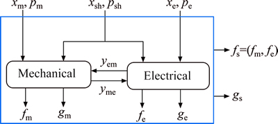
Fig. 1 A multi-physics microstructure with fully coupled two- discipline

The MOP in Eq. (3) relates the multi physical behavior of a structure with two disciplines resolved following the NDMO approach.

          (3)

In Eq. (3), x_sh and p_sh represent a vector of shared variables and uncontrolled parameters between two disciplines, respectively. The vector p_m and p_e describe the disciplinary uncontrolled parameters, with the superscript m and e referring to mechanical and electrical discipline, respectively. The vector Y_m and Y_e represent functions used to compute the mechanical y_me and electrical y_me coupling variables, respectively. In this optimization problem, each discipline has its associated disciplinary input design variables (x_m, x_e), and disciplinary output objectives functions (f_m, f_e) and constraints (g_m, g_e). The overall objective functions and constraints of the multi-physics microstructure are represented by f_s and g_s as shown in Fig. 1.

In order to assess the performance of each discipline individually, we use the suggested IMOCO approach for decomposing the NDMO problem of the multi-physics microstructure in Eq. (1) into two levels of optimization.

2.1 IMOCO approach

The presented multi-objective optimization approach for multi-physics microstructures is inspired from MOCO method [11]. IMOCO has several key properties and capabilities: it decomposes the MOP of fully coupled multi-physics microstructures according to the different disciplines that come into play in these microstructures, reduces computational effort, and it is suitable for solving multi-physics optimization problems.

In order to ensure the interdisciplinary compatibility after decomposition of all disciplines, we integrate Ref. [11] into the disciplinary objectives functions as follows.

Interdisciplinary consistency constraint C_ic of the mechanical discipline’s optimizer is given:

          (4)

Interdisciplinary consistency constraints of the electrical discipline’s optimizer are:

          (5)

Equations (4) and (5) are the expressions of the two interdisciplinary consistency constraints C_ic,m and C_ic,e of the mechanical and electrical discipline's optimizer, respectively. These constraints are reformulated integrated into the objective functions of the mechanical and electrical discipline, respectively. The interdisciplinary consistency constraint of mechanical discipline in Eq. (4) aims to minimize the difference between the shared variables generated in the mechanical discipline’s optimizer and the shared variables created at microstructure level. In addition, this constraint reduces the difference between the mechanical discipline coupling variable y_me (output of mechanical discipline) and the auxiliary variable obtained and sent from the microstructure level toward the mechanical discipline level, likewise the minimizing of the difference is performed between the local auxiliary variableand the auxiliary variable transferred from the microstructure level to the mechanical discipline level. A similar treatment is applied to the electrical discipline.

The application of the proposed IMOCO (see Fig. 2) approach on the optimization problem in Eq. (3) provides three-optimization problems: 1) one optimization problem at microstructure level in Eq. (6), and 2) two optimization problems at discipline level in Eqs. (7)-(8), and each level has its associated optimizer. Therefore, we have three optimizers: the microstructure level’s optimizer, the mechanical discipline’s optimizer, and the electrical discipline’s optimizer as shown in Fig. 2.

1) Microstructure level optimizer is

       (6)

In Eq. (6), the microstructure level objectives and constraints can be described as f_s and g_s, respectively. These microstructure objective and constraint functions depend on a vector X_s that contains the shared variables between the two disciplines and the auxiliary variablesThe vector P_s includes microstructure parameters P_s and microstructure level shared parameters The goal of the microstructure level optimizer is to optimize microstructure level objectives f_s with respect to microstructure design variables X_s subject to microstructure level constraints g_s. The superscript (*) indicates that the design variables are optimized at discipline level optimizer.

2) Mechanical discipline’s optimizer is

         (7)

The mechanical discipline optimizer in Eq. (7) aims to minimize the disciplinary objectives functions f_m limited by constraints g_m while respecting the design variable X_m, which includes mechanical optimizer variables x_m, shared variables and auxiliary (target) variables . The term P_m in Eq. (7) defines the mechanical optimizer parameters p_m and shared parameters p_sh.

3) Electrical discipline’s optimizer is

           (8)

Equally, the optimizer of the electrical discipline aims to reduce to a minimum the objectives functions f_e, which is associated with a number constraints g_e. In Eq. (8), the vector X_e represents a solution to this optimization problem, which includes electrical optimizer’s variables x_e, shared variablesand auxiliary (target) variablesThe term P_e represent electrical optimizer’s parameters p_e and shared parameters P_sh.

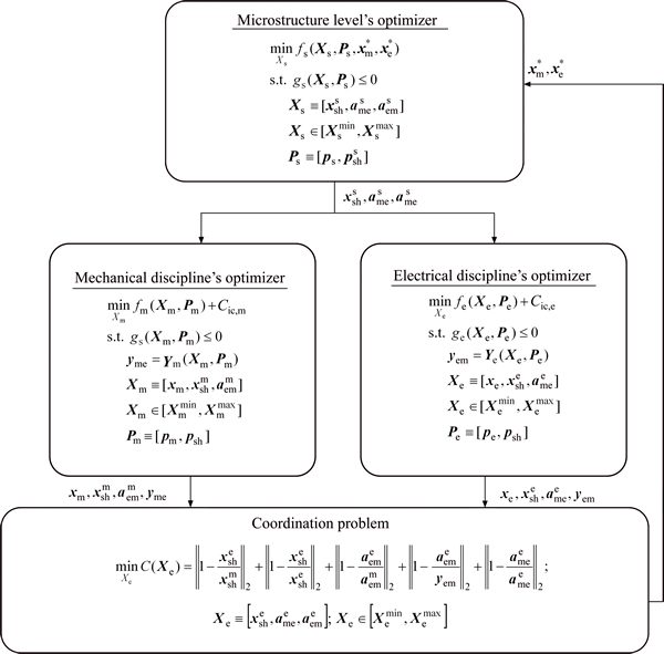
Fig. 2 Proposed IMOCO approach

In IMOCO method, each solution obtained at the microstructure level optimizer is sent to the discipline level optimizer and the disciplines are optimized for all design variables obtained at the microstructure level optimizer. In each iteration, the optimizer at discipline level has multiple solutions in the form of a Pareto optimal frontier. In order to assist each discipline selecting the best solution from its Pareto set, we introduce a coordination problem as in Eq. (9).

        (9)

The main objective of the coordination problem of Eq. (9) is to minimize the difference between the shared parameters transferred from each discipline level optimizer and the coordination shared variables The coordination problem is useful in minimizing the difference between the coordination auxiliary variables and the discipline level optimizer auxiliary parametersIn addition, it reduces the difference between the coordination auxiliary variables and the interdisciplinary coupling variables transferred from all disciplines level optimizer.

After the assessment of the coordination problem, we chose the disciplines’ optimal design variables with the minimum value of the single- objective function (see Eq. (9)) these variables are then passed to the optimizer at the microstructure level.

The steps involved in the implementation of the IMOCO are as follows.

Step 1: The microstructure level optimizer in Eq. (6) generates a set of values for, and in the initial generation.

Step 2: For each microstructure level design alternative, the values for are passed to each discipline level optimizer (mechanical discipline level optimizer in Eq. (7), and electrical discipline level optimizer in Eq. (8)).

Step 3: Each discipline level optimizer (Eqs. (7)- (8)) solves its associated optimization problem.

Step 4: The values for disciplinary design variables discipline level optimizer auxiliary variables and interdisciplinary coupling variables are passed from discipline level optimizer to the coordination problem (Eq. (9)) in order to choose the best solution.

Step 5: The selected optimal value from the coordination problem (Eq. (9)) are passed to the microstructure level optimizer (Eq. (6)).

Step 6: The microstructure level optimizer (Eq. (6)) then computes the microstructure’s objectives functions f_s subject to constraints g_s that depend on shared design variablesdisciplines optimal design variables and auxiliary variables

Step 7: The microstructure level optimizer (Eq. (6)) generates a new population for and .

Steps 2-7 are repeated until a stopping criterion is met. The stopping criterion is when a pre-specified maximum number of iterations is reached.

2.2 IMORCO approach

The Non-distributed MORO method in section 2 and IMOCO method are used here to develop the IMORCO approach. In IMORCO approach, the output variable from a discipline can be the input variable in another discipline; thus, allowing a variation range for an output variable, which creates an input uncertainty to another discipline. To overcome these shortcomings, the interdisciplinary propagation of uncertainty [12] is used in this work in order to ensure the collaborative robustness in IMORCO framework. The details of the IMORCO approach for the multi-physics microstructures and their disciplines optimization problems are presented below.

In this framework, the multi-physics microstructure’s optimization problem in Eq. (6) is solved as follows.

First, microstructure’s deterministic optimization is given:

             (10a)

Then, microstructure’s robustness assessment is given:

 (10b)

In the first step, a deterministic MOP, Eq. (10a), is solved to obtain a set of optimal solutions of the multi- physics microstructure. In a second step, a robustness assessment problem, Eq. (10b), uses the Pareto optimal solutions obtained in Eq. (10a) in order to find the WPPs. This is done by optimization over the vector of uncontrolled design parameters △P_s and △a_s.

The robustness of the optimal solution obtained from Eq. (10a) is checked through the constraint C_s≤0 of Eq. (10b). The distinct optimal solution is inserted in the set and then replaced in Eq. (10a). This creates “constraint cuts” used to restrict the feasible domain. In fact, the constraint C_s is used as a robustness indicator for optimal solutions.

We applied the same robustness assessment to both disciplines (mechanical in Eqs. (11a)-(11b), and electrical Eqs. (12a)-(12b); for both disciplines each MOP is decomposed into two stages in order to assess robustness.

First stage: Mechanical discipline’s deterministic optimization is given:

        (11a)

Second stage: Mechanical discipline’s robustness assessment is given:

                 (11b)

The mechanical discipline optimizer in Eq. (7) is divided into two optimization stages. The first is indicated in Eq. (11a) which aims to search the optimal solutions set; while in the second, the robustness assessment problem in Eq. (11b) aims to assess the robustness for each optimal solution obtained in Eq. (11a).

First stage: Electrical discipline’s deterministic optimization is given:

         (12a)

Second stage: Electrical discipline’s robustness assessment is given:

             (12b)

Similarly, the electrical discipline optimizer in Eq. (8) consists in two optimization steps. The first step, Eq. (12a), optimal solutions related to the electrical discipline are sought out; while in the second step, Eq. (12b), the robustness of each optimal solution obtained from Eq. (12a) is assessed.

3 Examples and results

To demonstrate our proposed approach, we treat two examples. The first one is a mathematical example, which contains two disciplines. The second one is an engineering example of CMUT type, which links three disciplines (mechanical, electrical and acoustic) and is more involved. The obtained results are compared with those obtained using the MOCO approach.

3.1 Mathematical example

The example is taken from a test case in Refs. [7, 11, 15] to validate our proposed approach. The two-objective optimization formulation for this problem, in the NDMO form is given in Eq. (13). The problem has two objectives functions (f₁, f₂) to optimize, which depend on six design variables, and subject to six inequality constraints.

(13)

In the nominal case, the IMOCO approach consists in decomposing the above problem into an optimization problem at the microstructure level (upper level) and two optimization problems at discipline levels 1 and 2 (lower level), as shown in Fig. 3.

The partition of the optimization problem in Eq. (13) by MOCO approach can be found in Ref. [11].

After solving the coordination problem (coordinator) in Fig. 3, we choose the optimal variables vector at the disciplinary levelwith the minimum value of this mono-objective problem and then their values are sent to the microstructure optimizer.

In the robustness framework, the uncertainty interval [△x₃, △x₆] of the design variables (x₃, x₆) is assumed to be within ±10% from nominal values, while the AOVRs for the objectives functions (△f_1.1, △f_1.2, △f_2.2) in Discipline 1 and Discipline 2 are ±20% of their nominal values. The problem in Eq. (13) can be decomposed according to our proposed IMORCOapproach as in Eqs. (10a)-(12b) into a problem at the upper-level in Eq. (14), and two problems in each discipline (1 and 2). The optimization problem of Discipline 1 in Fig. (3) is divided into two steps: 1) deterministic optimization problem in Eq. (15a), and 2) robustness assessment problem in Eq. (15b). Similarly, the optimization problem of Discipline 2 of Fig. 3 is also split into two optimization stages. In the first step, a deterministic optimization problem is solved; in the second step, the robustness of problem is assessed as shown in Eqs. (16a)-(16b).

Microstructure’s deterministic optimization is given:

    (14)

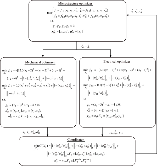
Fig. 3 Mathematical example decomposed in IMOCO framework

First stage: Discipline 1’s deterministic optimization:

        (15a)

Second stage: Discipline 1’s robustness assessment:

  (15b)

First stage: Discipline 2’s deterministic optimization:

      (16a)

Second stage: Discipline-2’s robustness assessment:

        (16b)

For the deterministic optimization, the obtained nominal Pareto set at the microstructure level using the MOCO and IMOCO approaches is represented in Fig. 4(a) and are compared to the reference (i.e., NDMO). Fig. 4(a) shows that Pareto optimal set of the IMOCO method is comparable with those from NDMO and MOCO. As shown, the IMOCO optimal solutions overlap with the NDMO and MOCO nominal Pareto frontier. This was also confirmed by the Mahalanobis distance[21] between NDMO and MOCO and between NDMO and IMOCO. To better compare the performance (precision and convergence time) of the IMOCO and the MOCO methods we used the OS metrics [22] to measure the precision and the CPU time to measure the speed of convergence. The results in Table 1 show the advantage of our proposed IMOCO method.

For robust optimization, the robust Pareto frontiers of the optimization problem at upper level in Eq. (14) by NDMORO, MORCO and IMORCO approach are shown in Fig. 4(b). As can be seen, the robust Pareto set obtained by the NDMORO approach is close to the nominal Pareto frontier. However, the robust Pareto frontier spreads along the nominal Pareto set, thus ensuring the robustness and optimality of the design variables at the same time. Consequently, the overlap of the robust Pareto set created by IMORCO is significantly better than the non-overlapping robust Pareto solutions from MORCO because not only is this frontier robust, but it also belongs to the nominal Pareto frontier. It can be seen that the robust Pareto frontier from IMORCO dominates (are better than) the robust Pareto solutions from MORCO. The MORCO approach uses the MOCO formulation from Ref. [11] with the addition of the robustness assessment criteria presented in Section 2. Results in Table 2 show the performance of the proposed IMORCO method compared to that of MORCO approach. Based on the results of this example, it can be seen that the deterministic and robust solutions obtained by the proposed IMOCO and IMORCO respectively are consistent with NDMO and NDMORO.

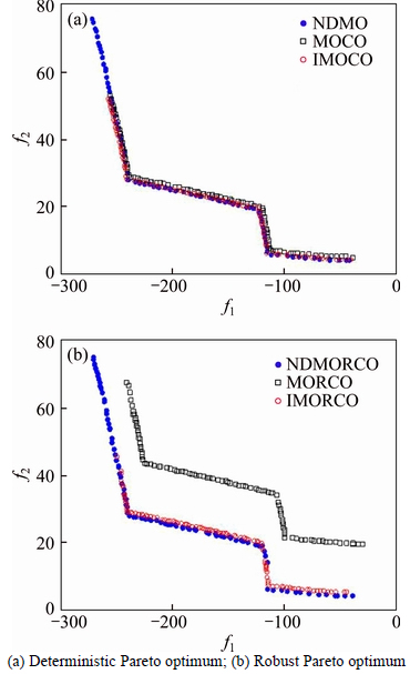
Fig. 4 Feasible objective space for numerical example:

Table 1 Performance of proposed IMOCO method vs MOCO method

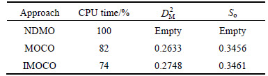
Table 2 Performance of proposed IMORCO method vs MORCO method

3.2 Engineering example: CMUT

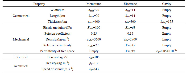
After validation of our original approaches, we took an engineering example of CMUT [23] type to demonstrate the efficiency and accuracy of our proposed method. It is a multi-physics microstructure, which involves the nonlinear coupling between three physics:mechanical, electrical, and acoustical. Due to the electro-mechano-acoustic, nonlinear coupling of this MEMS type, the optimization process is most likely difficult. In fact, it requires several cycles of finite element analysis. In this section, a genetic algorithm NSGA-II type is coupled with finite element model, i.e., without approximation tools in order to increase the efficiency of the CMUT cell. Figures 5(a)-(b) show the geometry of the moveable part of a CMUT cell and the boundary conditions used, respectively. The CMUT cell is biased with a constant voltage value (V_dc) thus creating an electrostatic pressure (P_ele), which causes a displacement of the membrane. This movement generates a radiated pressure (P_rad) in the fluid on the front side of the membrane. Table 3 lists the geometrical, mechanical, electrical and the acoustical properties of the CMUT cell.

The MOP of the CMUT cell to solve following the NDMO approach is given in Eq. (17). It has three objective functions, nine design variables and four inequality constraints: 1) minimize the mechanical resonance frequency of a CMUT cell (f_rm(x)), 2) maximize the electromechanical coupling coefficient and 3) maximize the average velocity (V_avr(x)).

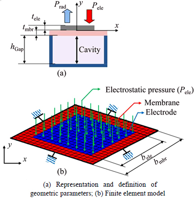
Fig. 5 CMUT cell:

Table 3 Geometrical, mechanical, electrical and acoustical properties used in finite element simulations of CMUT cell [23]

The MOMPO problem to solve is then:

(17)

In this part, the MOMPO problem in Eq. (17) can be decomposed into two levels of optimization; 1) microstructure level (CMUT cell), and 2) discipline level (mechanical, electrical and acoustical using the proposed IMOCO approach. While each discipline has its own design variables, five design variables are shared between the microstructure level and discipline level,

they are The first four-design variables are shared between the microstructure (CMUT cell) and the three disciplines (mechanical, electrical and acoustic); and the last design variable (ρ_mbr) is shared between the mechanical and acoustic disciplines.

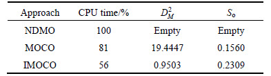
In the nominal case, Fig. 6 shows three dimensions of the nominal Pareto frontier obtained by the reference, i.e., NDMO, MOCO and IMOCO. It can be seen that the Pareto solutions produced by IMOCO overlaps with the NDMO Pareto frontier and does not overlap with the MOCO nominal Pareto frontier. This is also confirmed by the Mahalanobis distance between NDMO and MOCO and between NDMO and IMOCO. It can be observed in Table 4 that the CPU time, the values for and OS from the IMOCO are better than MOCO.

In a robustness framework, the uncertainty interval of the design variables are assumed to be within ±5% of their nominal values. The AOVRs for the objectives functionsare 20% of their nominal values. The tolerance regions of the auxiliary variables a_em are within ±1%. The AOVR for the coupling variables is 20% of the nominal values.

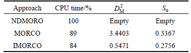
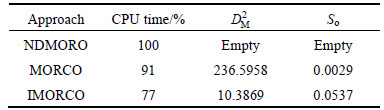
The optimization problem at the microstructure level has been solved using NDMORO, MORCO and IMORCO approaches and their robust Pareto frontiers are shown in Fig. 7. It is clear that the robust Pareto frontier produced by IMORCO converge to NDMORO robust solutions but the obtained robust Pareto solutions by MORCO do not coincide with NDMORO robust optimal solutions. From Table 5, we can see that the CPU time, the values for and OS from the IMORCO are better than MORCO.

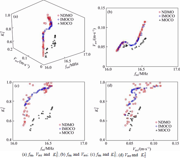
Fig. 6 Feasible pareto optimal solutions for engineering example in plane:

Table 4 Performance of proposed IMOCO method vs MOCO method

4 Conclusions

1) A new two-level multi-objective optimization approach in CO framework is developed to handle the multi-physics microstructures with several disciplines fully coupled and multiple objectives/ constraints at the microstructure and discipline levels. First, the IMOCO approach aims to find the Pareto optimal frontier for multi-physics and multi-objective optimization problems of multi-physics microstructures. Second, the IMORCO approach achieves the same task taking into consideration interval uncertainty. In these two original approaches, a coordination problem is introduced between the upper and lower level, which minimizes the difference between the shared and the coupling variables transmitted from all disciplines in order to avoid discrepancy during optimization. We applied these original approaches to a mathematical example and an engineering example CMUT cell type. The obtained results are compared with the previous methods.

2) In the first example, it is observed in the nominal case that there is a good agreement between the Pareto optimal frontiers obtained by NDMO and by proposed IMOCO. This is also confirmed by the Mahalanobis distance (=0.2748) and the OS metrics (OS=0.3461). In this example, the IMOCO approach leads to a reduced CPU time by 26%. For the robust case, the Mahalanobis distance (=0.5471) and the OS metrics (OS=0.2756) confirm that the robust Pareto set created by the proposed IMORCO approach close to the robust Pareto frontier obtained by NDMORO. In addition, the CPU time is decreased by 16% in this robust optimization.

3) In the CMUT cell type example, it is observed a significant overlap between optimal Pareto frontiers obtained by NDMO and IMOCO approaches,respectively. This overlap is confirmed by the Mahalanobis distance (=0.9503) and the OS metrics (OS=0.2309). The IMOCO allows us to reduce the CPU time by 44%. In addition, the consideration of robustness in IMORCO approach applied to a CMUT cell of optimization problem under interval uncertainty has reduced the CPU time by 23% keeping a robust Pareto front overlaps with that obtained by the robust NDMORO approach (=10.3869 and OS=0.0537).

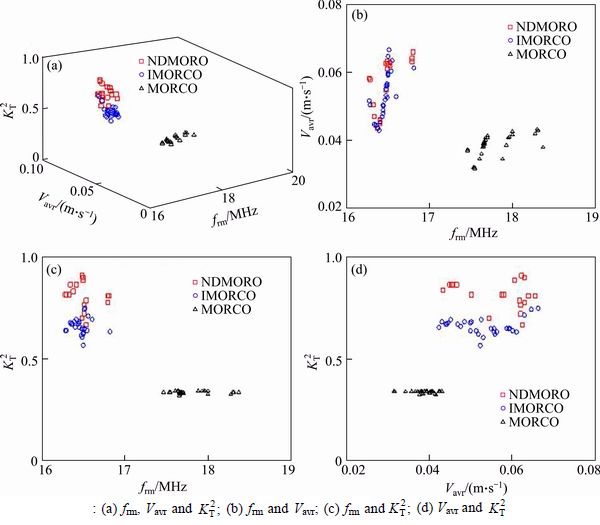
Fig. 7 Robust feasible pareto optimal solutions for engineering example in plane:

Table 5 Performance of proposed IMORCO method vs MORCO method

4) Finally, it could be concluded that IMOCO and IMORCO approaches provide solutions that are consistent optimal and robust solutions respectively with the NDMO and NDMORO methods. These proposed two methods require less computational efforts than the previous approaches.

Nomenclature

AOVR

Acceptable objective variation range

CO

Collaborative optimization

CMUT

Capacitive micromachined ultrasonic

transducers

CPU

Computer run time

IMOCO

Improved multi-objective collaborative

optimization

IMORCO

Improved multi-objective robust

collaborative optimization

MCRO

Multi-objective collaborative Robust

optimization

MDO

Multidisciplinary design optimization

MOCO

Multi-objective collaborative

optimization

MPMO

Multi-physics multi-objective

optimization

MOP

Multi-objective Optimization Problem

MORCO

Multi-objective robust collaborative optimization

MORO

Multi-objective robust optimization

NDMO

Non-distributed multi-objective

optimization

NDMORO

Non-distributed multi-objective robust optimization

NSGA-II

Non-dominated sorting genetic

algorithm-II

OS

Overall spread

Vector of auxiliary design variable with output from an electrical discipline (e) and input to mechanical discipline (m), generated in mechanical discipline (m) (in Eq. (4))

Auxiliary design vector with output from a mechanical discipline (m) and input to electrical discipline (e), generated in electrical discipline (e) (in Eq. (5))

Vector of auxiliary design variable with output from an electrical discipline (e) and input to mechanical discipline (m), generated in microstructure level (s) (in Eq. (4))

Auxiliary design vector that is output of mechanical discipline and input to electrical discipline (e), generated in in microstructure level (s) (in Eq. (5))

n_f

Number of objective functions (in Eq. (2a))

n_g

Number of constraint functions (in Eq. (2a))

S_WPP

Set of worst possible points (in Eq. (2a))

u_dc

Static deflection of the membrane (in Eq. (17))

△f_e

AOVR for electrical discipline level objective (in Eq. (12b))

△f_m

AOVR for mechanical discipline level objective (in Eq. (11b))

△f_s

AOVR for microstructure level objective (in Eq. (10b))

△y_em

AOVR for electrical-mechanical coupling variables (in Eq. (11a))

△y_me

AOVR mechanical-electrical coupling variables (in Eq. (12a))

L₂ norm

References

[1] BALLING R J, SOBIESZCZANSKI-SOBIESKI J. Optimization of coupled systems—A critical overview of approaches [J]. American Institute of Aeronautics and Astronautics Journal, 1996, 34(1): 6-17.

[2] BALESDENT M, P, CHRIETTE A. A survey of multidisciplinary design optimization methods in launch vehicle design [J]. Structural and Multidisciplinary Optimization, 2011, 45(5): 619-642.

[3] TAPPETA R V, RENAUD J E. Multiobjective collaborative optimization [J]. Journal of Mechanical Design, 1997, 119(3): 403-411.

[4] BRAUN R D, KROO I M. Development and application of the collaborative optimization architecture in a multidisciplinary design environment [J]. Multidisciplinary Design Optimization: State of the Art, Society for Industrial and Applied Mathematics, 1996, 1: 98-116.

[5] SOBIESZCZANSKI-SOBIESKI J. Optimization by decomposition: A step from hierarchic to non-hierarchic systems [C]// NASA/Air Force Symposium on Recent Advances in Multidisciplinary Analysis and Optimization. Hampton, Virginia: NASA Press, 1989: 51-78.

[6] KIM M H, MICHELENA N F, PAPALAMBROS P Y, JIANG T. Target cascading in optimal system design [J]. Journal of Mechanical Design, 2003, 125(3): 474-480.

[7] DEB K. Multi-objective optimization using evolutionary algorithms [M]. New York: John Wiley & Sons, 2001: 227-351.

[8] DOERNER K, GUTJAHR W J, HARTL R F, STRAUSS C, STUMMER C. Pareto ant colony optimization: A metaheuristic approach to multiobjective portfolio selection [J]. Annals of Operations Research, 2004, 131(1/2/3/4): 79-99.

[9] KENNEDY J, EBERHART R. Particle swarm optimization [C]//IEEE International Conference on Neural Networks Proceedings. Washington: IEEE Press, 1995, 4: 1942-1948.

[10] GILL P, MURRAY W, SAUNDERS M. Large-scale SQP methods and their application in trajectory optimization [C]// ISNM International Series of Numerical Mathematics. San Francisco: Springer Press, 1994: 29-42.

[11] AUTE V, AZARM S. Genetic algorithms based approach for multidisciplinary multiobjective collaborative optimization [C]// AIAA/ISSMO Multidisciplinary Analysis and Optimization Conference. Portsmouth, Virginia: AIAA Press, 2006: 1-17.

[12] LEE J. A structural design of multilevel decomposition and domain mapping [J]. Journal of Central South University, 2014, 21(9): 3504-3512.

[13] YANG H D, E J O, QU T. Multidisciplinary design optimization for air-condition production system based on multi- agent technique [J]. Journal of Central South University, 2012, 19(2): 527-536.

[14] LI M, AZARM S. Multiobjective collaborative robust optimization with interval uncertainty and interdisciplinary uncertainty propagation [J]. Journal of Mechanical Design, 2008, 130(8): 719-729.

[15] LI H, MA M X, JING Y W. A new method based on LPP and NSGA-II for multiobjective robust collaborative optimization [J]. Journal of Mechanical Science and Technology, 2011, 25(5): 1071-1079.

[16] HU W W, AZARM S, ALMANSOORI A. New approximation assisted multi-objective collaborative robust optimization (new AA-McRO) under interval uncertainty [J]. Structural and Multidisciplinary Optimization, 2013, 47(1): 19-35.

[17] XIONG F, SUN G R, XIONG Y, YANG S X. A moment-matching robust collaborative optimization method [J]. Journal of Mechanical Science and Technology, 2014, 28(4): 1365-1372.

[18] GUNAWAN S, AZARM S. Multi-objective robust optimization using a sensitivity region concept [J]. Structural and Multidisciplinary Optimization, 2004, 29(1): 50-60.

[19] HU W, LI M, AZARM S, al HASHIMI S, ALMANSOORI A, al QASAS N. Improving multi-objective robust optimization under interval uncertainty using worst possible point constraint cuts [C]// ASME International Design Engineering Technical Conferences and Computers and Information in Engineering Conference. California: ASME Press, 2009: 1193-1203.

[20] GUNAWAN S, AZARM S. Non-gradient based parameter sensitivity estimation for robust design optimization [J]. Journal of Mechanical Design, 2004, 126(3): 395-402.

[21] de MAESSCHALCK R, JOUAN-RIMBAUD D, MASSART D L. The mahalanobis distance [J]. Chemometrics and Intelligent Laboratory Systems, 2000, 50(1): 1-18.

[22] WU J, AZARM S. Metrics for quality assessment of a multi-objective design optimization solution set [J]. Journal of Mechanical Design, 2000, 123(1): 18-25.

[23] MEYNIER C, TESTON F, CERTON D. A multiscale model for array of capacitive micromachined ultrasonic transducers [J]. Journal Acoustical Society of America, 2010, 128(5): 2549-2561.

(Edited by FANG Jing-hua)

Received date: 2015-11-03; Accepted date: 2016-02-01

Corresponding author: Hamda Chagraoui, PhD; Tel: +216-97-207589; fax: +216-71391166; E-mail: hmdchagraoui@gmail.com