J. Cent. South Univ. (2012) 19: 651-656

DOI: 10.1007/s11771-012-1052-z

Analytical models for evaluating buoyancy-driven ventilation due to

stack effect in a shaft considering heat transfer from shaft interior boundaries

YANG Dong(阳东), LI Bai-zhan(李百战), DU Tao(杜涛), LI Nan(李楠)

Faculty of Urban Construction and Environmental Engineering, Chongqing University, Chongqing 400045, China

? Central South University Press and Springer-Verlag Berlin Heidelberg 2012

Abstract: Stack effect is a dominant driving force for building natural ventilation. Analytical models were developed for the evaluation of stack effect in a shaft, accounting for the heat transfer from shaft interior boundaries. Both the conditions with constant heat flux from boundaries to the airflow and the ones with constant boundary temperature were considered. The prediction capabilities of these analytical models were evaluated by using large eddy simulation (LES) for a hypothetical shaft. The results show that there are fairly good agreements between the predictions of the analytical models and the LES predictions in mass flow rate, vertical temperatures profile and pressure difference as well. Both the results of analytical models and LES show that the neutral plane could locate higher than one half of the shaft height when the upper opening area is identical with the lower opening area. Further, it is also shown that the analytical models perform better than KLOTE’s model does in the mass flow rate prediction.

Key words: stack effect; theoretical analysis; large eddy simulation; vertical temperature distribution; heat transfer

1 Introduction

Nowadays, buildings consume roughly 40% of the energy use [1]. Building energy conservation has consequently become an important concern. One strategy for decreasing building energy consumption is to use natural ventilation [2]. The use of stack effect is one of the most feasible strategies in natural ventilation design [3-7]. This strategy utilizes buoyancy as the driving force for ventilation when the air inside the building is warmer than the ambient. Due to the importance of stack effect in natural ventilation design, it is essential to have suitable tools to predict its performance or its relevant parameters for an actual building, e.g., the location of neutral plane and the air mass flow rate induced by stack effect.

Some analytical models have already been proposed to predict the mass flow rate due to stack effect [8-9]. The model developed by KLOTE [9], i.e., , with T denoting the absolute temperature of airflow inside the shaft and  denoting the height of neutral plane, is a well-known model, which is also recommended by the ASHRAE handbook [10]. It is shown from this model that the airflow temperature inside the shaft is one of the primary factors that determine the magnitude of stack effect. In addition, KLOTE’s model indicates that the height of neutral plane is always less than one half of the total shaft height if the opening of the upper vent is identical with that of the lower vent [9]. However, KLOTE’s model simplified the airflow temperature inside the shaft as a uniform one. It should be noted that there could be heat exchange between the warmer shaft interior boundaries and the cooler airflow flowing through the shaft in some conditions (see Fig. 1), due to the operation of heating system or the exhausted gas being discharged into the shaft. The heat transfer between the boundary and the airflow results in the increase in airflow temperature. This could also be the reason for the air inside the shaft being warmer than the outside one. For a relatively high shaft, the heat transfer from interior boundaries would result in the airflow temperature varying appreciably with elevation, as shown in Ref. [11]. In this sense, the traditional model, which neglects the variation in  airflow temperature in the vertical direction, could be difficult to provide reasonable results for such conditions. This indicates that further work is necessary on this topic.

In principle, there is no problem in performing computational fluid dynamics (CFD) to evaluate stack effect in such conditions [12-14]. Both the mass flow rate and the location of neutral plane can be solved by implementation of CFD when the thermal boundary conditions are accurately prescribed. However, practical problem may arise when the shaft is very long. The number of grid cells becomes numerous in such long configurations, which raises the computational cost or even prohibits the CFD simulation. One way of circumventing this problem is to use simplified analysis with consideration of heat exchange between the airflow and shaft interior boundaries. The latter approach is in general sufficient for evaluation of stack effect as engineering purpose, and would be more accurate than the traditional model (i.e., the KLOTE’s model) from physical insights. This motivates the study presented in the current work.

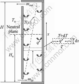
Fig. 1 Schematic diagram of natural ventilation due to stack effect in shaft with heat transfer from shaft interior boundaries

In this work, analytical models were developed for evaluation of stack effect in a vertical shaft, with taking the heat transfer from shaft interior boundaries to airflow into account. These models are derived from fundamental equations of fluid dynamics and energy balance. Two typical thermal boundary conditions are considered. The first one is the case with constant heat flux from boundaries, and the other is the case with constant boundary temperature. The analytical model predictions are then compared against the large eddy simulation (LES) results for validation purpose.

2 Theoretical analysis

2.1 Assumptions

The analytical model is one-dimensional: all quantities are averaged over the shaft cross-section. The following assumptions are made:

1) The ambient temperature and the thermal boundary inside the shaft do not vary in time and thus remain equal to their initial values; the ambient air density varies little with elevation;

2) The airflow follows the ideal gas law and the gas constant R is a constant value;

3) The viscosity of airflow near the wall is very small and thus the boundary layers of temperature and velocity are neglected;

4) The airflow in the shaft is considered to be one-dimensional in the vertical direction;

5) The heat transfer from boundaries to the airflows is simplified as a convective process and the convective heat transfer coefficient is assumed to be constant.

2.2 Case with constant heat flux from shaft interior boundaries

The magnitude of stack effect is strongly dependent on the airflow temperature inside the shaft. The energy equation for the control volume shown in Fig. 1 is given as

                              (1)

where q″ is the convective heat flux from boundaries, S is the length of heating section in the cross plane, c_p is the heat capability,  is the mass flow rate due to stack effect, T is the airflow temperature and x is the coordinate in the vertical direction.

The temperature difference between airflow temperature and ambient one, ?T, is introduced, then Eq.(1) can be rewritten as

                           (2)

Combining with the boundary condition:

                                  (3)

it gives

                                   (4)

with

                                  (5)

It is deduced from Eq. (4) that the airflow temperature linearly increases with elevation. Thus, the airflow density varies with elevation as well. If the upper opening locates at the top of the shaft, the flow out of the upper opening is

                  (6)

where  is the mass flow rate out of the upper opening, C is the flow coefficient, A_u is the area of upper opening,  is the pressure difference at the upper opening, ρ_u is the gas density at the upper opening, ρ_a is the ambient air density, ρ_g is the local gas density in the shaft, g is the gravitational acceleration constant, H_n is the height of neutral plane, and H_u is the height of the upper opening.

Substituting Eq. (4) into Eq. (6) and applying the ideal gas law in Eq. (6), it yields

(7)

If the lower opening locates at the bottom of the shaft, the air flow into the lower opening is

    (8)

where  is the mass flow rate through the lower opening, A_l is the area of lower opening, and H_l is the height of the lower opening.

For steady flow, the flow out of the shaft should be equal to the one into the shaft. H_n and  can then be obtained by combing Eq. (7) and Eq. (8). This non-linear equation system can be numerically solved by using iterative approach, such as the Newton-Raphson method.

2.3 Case with constant boundary temperature

For the case with constant boundary temperature, the energy equation can also be represented as Eq. (1). The convective heat flux q″ is

                        (9)

where ?T_w is the temperature difference between wall and airflow, and h is the convective heat transfer coefficient.

Combining with the boundary condition:

                    (10)

it gives

                          (11)

with

                                  (12)

It is deduced from Eq. (11) that the airflow temperature follows an exponential decay vertically in such conditions.

Combing with the ideal gas law, the flow out of the upper opening is

        (13)

The flow into the lower opening is

(14)

For steady flows, H_n and  can be calculated by combing Eq. (13) and Eq. (14).

3 Comparison with LES predictions

The analytical models were applied into a hypothetical shaft with a dimension of 304 m (height)× 20 m (length)×2 m (width), as shown in Fig. 2. The shaft was connected to the outside space through two vertical openings. The lower opening was located at the height of 2 m and the upper one was located at the height of 303 m. Both openings have a dimension of 2 m (width)×1 m (height), as shown in Fig. 2. The case with constant heat flux from boundaries and the one with constant boundary temperature were both considered. The ambient temperature was 10 °C. For both cases, the thermal boundary conditions were prescribed at the walls parallel with the opening, and all the other boundary walls were set to be adiabatic, as shown in Fig. 2. The computational domain was extended to be 400 m (height)×60 m (length)×2 m (width).

The boundary conditions for these two cases are illustrated in Table 1 and Table 2, respectively. Large eddy simulation was also implemented to simulate the same scenarios by using fire dynamics simulator (FDS) [15]. The thermally-driven flows were numerically solved, in combination with the classical Smagorinsky model as a sub-grid scale (SGS) model for turbulence modeling [9]. Two-dimensional simulations were performed by using uniform rectangular grid cells with size of 1 m (height)×1 m (length)×2 m (width). Both the results of the analytical model of this work and the KLOTE’s model are compared against the LES predictions.

Figure 3 shows the temperature counters and pressure difference counters predicted by LES at the middle plane for Case 1. The vertical profiles of temperature and pressure difference predicted by the analytical models were compared against the LES predictions. It is shown from Fig. 3 that the airflow temperature generally increases with elevation. Figure 4 shows the profile of temperature rise predicted by this analytical model and the one predicted by LES for Case 1. The LES predictions correspond to the ones at the center of the cross plane during the steady period. It is shown that the analytical model predicts the temperature rise to increase more rapidly with elevation than LES does. The reason for this will be explained later. However, it is shown that the absolute temperature at the top of shaft predicted by the analytical model is only 4% higher than the LES prediction. This indicates that this analytical model has an acceptable capability for engineering design. Figure 5 shows the vertical distribution of pressure difference predicted by the analytical model and the one predicted by LES for Case 1. It is shown that these two pressure profiles get fairly good agreement. The neutral plane with zero pressure difference predicted by the analytical model is higher than the one obtained from LES.

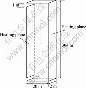
Fig. 2 Schematic diagram of hypothetical two-vent shaft with heat transfer from interior boundaries

Table 1 Simulation scenarios and results of LES, KLOTE’s model and model accounting for heat transfer for Case 1

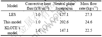
Table 2 Simulation scenarios and results of LES, KLOTE’s model and model accounting for heat transfer for Case 2

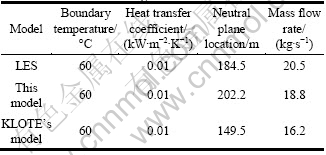
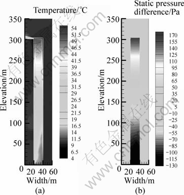
Fig. 3 LES predictions of temperature distribution (a) and pressure distribution (b) at central plane

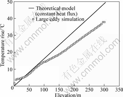
Fig. 4 Comparison of vertical temperature profile predicted by analytical model with LES prediction for Case 1

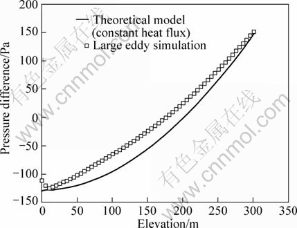
Fig. 5 Comparison of vertical pressure profile predicted by analytical model with LES prediction for Case 1

Figure 6 compares the profile of temperature difference between air density inside the shaft and the bounded wall, ?T_w, predicted by the analytical model with the one predicted by LES for Case 2. It is shown that ?T_w decreases more slowly with the elevation in the analytical model prediction than in the LES prediction. This indicates that the airflow temperature increases more rapidly with elevation in the analytical model than in the LES prediction. However, the deviation is only   6 °C at the top of the shaft. Figure 7 shows the vertical profile of pressure difference predicted by the analytical model and the one predicted by LES for Case 2. Although the neutral plane predicted by the theoretical model is higher than the one obtained from LES, these two profiles get fairly good agreement.

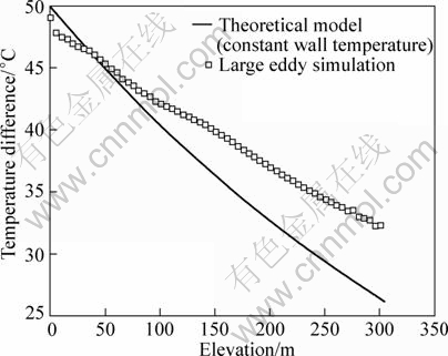
Fig. 6 Comparison of vertical temperature profile predicted by analytical model with LES prediction for Case 2

Fig. 7 Comparison of vertical pressure profile predicted by analytical model with LES prediction for Case 2

The two most important parameters related to stack effect, i.e., the mass flow rate into the shaft and the location of neutral plane, predicted by the analytical models of this work, KLOTE’s model and LES are all presented in Table 1 and Table 2. The average temperatures inside the shaft are obtained by spatially integrating the LES predicted temperature along the vertical direction. These integral average temperatures are used as the input parameters for the KLOTE’s model. It is shown from Table 1 that the location of neutral plane predicted by the analytical model of this work is higher than that predicted by LES for Case 1, with the deviation of 14%. However, the location of neutral plane predicted by the KLOTE’s model is lower than that predicted by LES for Case 1, with the deviation of 17%. It is also shown that the KLOTE’s model predicting the height of neutral plane is lower than one half of the shaft height, but both the LES and the analytical model of this work predict the neutral plane to be higher than one half of the shaft height. The mass flow rate into the shaft predicted by the analytical model is a little smaller than the one predicted by LES, with deviation of 10%. As shown in Eq. (4), the growth rate of temperature rise with elevation is inversely proportional to the mass flow rate. This must be the reason for that the temperature rise increases more rapidly with elevation in the analytical model predictions. It is also noted that the analytical model of this work performs better than KLOTE’s model in mass flow rate prediction. This is due to the fact that the KLOTE’s model neglects the temperature variation in the vertical direction.

For Case 2, the location of neutral plane predicted by the analytical model is still higher than the one predicted by LES (as shown in Table 2), with the deviation of 9%. The location of neutral plane predicted by the KLOTE’s model is lower than that predicted by LES for Case 2, with the deviation of 19%. The mass flow rate into the shaft predicted by analytical model is smaller than the one predicted by LES by about 8%, but the results are better than those of KLOTE’s model.

4 Conclusions

1) Analytical models for stack effect are developed with consideration of heat exchange between shaft interior boundary and air flow.

2) Heat transfer from shaft interior boundary has a strong impact on the location of neutral plane and mass flow rate through the shaft. There are fairly good agreements between the predictions of the analytical models and the LES predictions in mass flow rate, vertical temperatures profile and pressure difference.

3) The analytical models of this work perform better than the KLOTE’s model in both mass flow rate prediction and neutral plane location prediction. Both the results of analytical models and LES show that the neutral plane could locate higher than one half of the shaft height when the upper opening area is identical with the lower opening area. However, the KLOTE’s model predicts the location of neutral plane to be lower than one half of the shaft, due to neglecting the temperature variation in the vertical direction.

References

[1] DODOO A, GUSTAVSSON L, SATHRE R. Building energy-efficiency standards in a life cycle primary energy perspective [J]. Energy and Buildings, 2011, 43(7): 1589-1597.

[2] CIBSE. Natural ventilation in non-domestic buildings [R]. London: Chartered Institution of Building Services Engineers, 2005.

[3] ANDERSON K T. Theoretical consideration on natural ventilation by thermal buoyancy [J]. ASHRAE Technical Data Bulletin, 1995, 11(3): 48-62.

[4] BANSAL N K, MATHUR R, BHANDARI M S. Solar chimney for enhanced stack ventilation [J]. Building and Environment, 1993, 28(3): 373-377.

[5] BAROZZI G S, IMBABI M S E, NOBILE E, SOUSA A C M. Physical and numerical modelling of a solar chimney based ventilation system for buildings [J]. Building and Environment, 1992, 27(4): 433-445.

[6] van der MASS J, ROULET C A. Night time ventilation by stack effect [J]. ASHRAE Technical Data Bulletin, 1991, 7(1): 23-38.

[7] WONG N H, HERYANTO S. The study of active stack effect to enhance natural ventilation using wind tunnel and computational fluid dynamics (CFD) simulations [J]. Energy and Buildings, 2004, 36: 668-678.

[8] SHERMAN M H. Single-zone stack-dominated infiltration modeling [C]//Proceedings of the 12th IEA Conference of the Air Infiltration and Ventilation Centre. Ottawa, ON, 1991: 297-314.

[9] KLOTE J H. A general routine of analyzing of stack effect [R]. National Institute of Standards and Technology, NISTIR 4588, 1991.

[10] ASHRAE Handbook-fundamentals [R]. Inc Atlanta: American Society of Heating, Refrigerating and Air-Conditioning Engineers, 1997.

[11] KOTANI H, SATOH R, YAMANAKA T. Natural ventilation of light well in high-rise apartment building [J]. Energy and Buildings, 2003, 35: 427-434.

[12] LIM T, CHO J, KIM B S. Predictions and measurements of the stack effect on indoor airborne virus transmission in a high-rise hospital building [J]. Building and Environment, 2011, 46(12): 2413-2424.

[13] MAATOUK K, ASMA A. Stack pressure and airflow movement in high and medium rise buildings [J]. Energy Procedia, 2011, 6: 422-431.

[14] XIAO G Q, TU J Y, YEOH G H. Numerical simulation of the migration of hot gases in open vertical shaft [J]. Applied Thermal Engineering, 2008, 28: 478-487.

[15] MCGRATTAN K, HOSTIKKA S, FLOYD J, BAUM H, REHM R. Fire dynamics simulator (Version5)-Technical reference guide [R]. National Institute of Standards and Technology, 2007: 1018-1025.

(Edited by YANG Bing)

Foundation item: Project(50838009) supported by the National Natural Science Foundation of China; Project(2010DFA72740-03) supported by the National Key Technology Research and Development Program of China

Received date: 2011-07-26; Accepted date: 2011-11-14

Corresponding author: YANG Dong; Tel: +86-23-65120750; Fax: +86-23-65120773; E-mail: yangd8210@gmail.com, yangdong@cqu.edu.cn