J. Cent. South Univ. (2012) 19: 2689-2696

DOI: 10.1007/s11771-012-1328-3

Cascade control based on minimum sensitivity in outer loop for processes with time delay

YIN Cheng-qiang(尹成强)¹, HUI Hong-zhong(惠鸿忠)¹, YUE Ji-guang(岳继光)²,

GAO Jie(高洁)¹, ZHENG Li-ping(郑丽萍)³

1. School of Automobile and Transportation Engineering, Liaocheng University, Liaocheng 252059, China;

2. College of Electronics and Information Engineer, Tongji University, Shanghai 201804, China;

3. School of Computer Science, Liaocheng University, Liaocheng 252059, China

? Central South University Press and Springer-Verlag Berlin Heidelberg 2012

Abstract: A new cascade control program was proposed based on modified internal model control to handle stable, unstable and integrating processes with time delay. The program had totally four controllers of which the secondary loop had two controllers and the primary loop had two controllers. The two secondary loop controllers were designed using IMC technique. They were decoupled completely and could be adjusted independently, which avoided the undesirable influence on performance of the primary controllers. The main controller in the primary loop was devised as a PID using the method of minimum sensitivity, which could guarantee not only the nominal performance but also the robust stability of the system. A setpoint filter was added in the primary loop to improve the tracking performance. All the controllers of the two closed-loops were designed analytically, and could be adjusted and optimized by single parameter respectively. Simulations were carried out on three various processes with time delay, and the results show that the proposed method can provide a better performance of both set-point tracking and disturbance rejection and robustness against parameters perturbation.

Key words: cascade control; time delay; H_∞ performance specification; modified internal mode control; multiple degrees of freedom

1 Introduction

Cascade control is an alternative to conventional single feedback control to improve the performance of a control system. It is prior to be adopted for improving the system performance of load disturbance rejection under the condition that the intermediate process measurement can be conveniently obtained in practice. The advantages of easy implementation and potentially large control performance improvement have led to widespread applications of cascade control for several decades [1-2]. Generally, a cascade control structure consists of two control loops: a secondary intermediate loop and a primary outer loop. The idea of cascade structure is that the disturbances introduced in the inner loop are reduced to a greater extent in the inner loop itself before they extend into the outer loop [3].

As cascade structure includes two controllers, its tuning is more complicated than that of a standard single-loop. Therefore, some bibliographies about tuning methods have been published. For example, TAN [4] proposed tuning rules for the primary and secondary controllers based on performing the identification for the inner loop once the inner controller steps into place. In Ref. [5], a completely automated design procedure within the framework of the usual PI/PID controllers was presented. In Ref. [6], a design approach for two-degree-of-freedom PID controllers within a cascade control configuration guaranteeing robust and smooth control was presented and achieved better control performance. Another research area is modifying control structures based on a conventional cascade configuration, and the improvement comes from the fact that internal model controller or (and) Smith predictor scheme is used in the inner or outer loop. IBRAHIM et al [7] proposed a cascade control scheme combined with Smith predictor and really achieved better control performance compared with some existing conventional PID tuning methods. LIU et al [8] proposed a new two-degree-of-freedom control structure for cascade control systems, and illustrative examples demonstrated the superiority of the method.

However, the above-mentioned methods only considered the stable processes by either tuning methods or modified structure. Usually, there are some open-loop unstable and integrating processes with time delay in many industrial and chemical processes [3, 9-10]. For open-loop unstable processes, the water bed effect between the set point tracking and load disturbance rejection using a closed-loop control structure becomes severe no matter how the primary controller is tuned [11], and control of integrating systems with large time delay is a challenging and interesting task. LEE et al [12] modified the conventional cascade control structure by adding two filters to the set points of the inner and outer loops, respectively, and tuned the closed-loop controllers according to the internal model control theory, so that the load disturbance rejection performance was enhanced in comparison with some existing methods based on the conventional cascade control structure. Recently, IBRAHIM and DEREK [13] proposed a new cascade control structure and controller design based on standard forms for controlling unstable or integrating processes. DOLA and SOMANATH [14] proposed a modified Smith predictor for controlling open-loop unstable time delay processes, and there are only three controllers. In contrast to the conventional cascade control structure, parallel cascade control structures for some chemical processes were proposed [15-17].

In the conventional cascade systems, there is a trade-off between the response of the set-point tracking and load disturbance rejection responses in the secondary loop. Sometimes, the performance of the disturbance rejection in the primary loop depends on not only the disturbance rejection in the secondary loop but also the set point tracking in the secondary loop [17]. To improve system performance, in this work, an analytical control scheme is proposed.

2 Controller design procedure

The proposed control structure is shown in Fig. 1, where C₁(s) is the close loop controller in the primary loop; F₁(s) is the set-point filter of the primary loop; C₂(s) is the secondary controller in the inner loop used for set-point tacking; C₃(s) is the secondary controller in the inner loop used for rejecting load disturbances that seep into the intermediate process; P_2m is the model of the intermediate process P₂(s), and P₁(s) is the primary process; r₁(s) is the set point for the primary loop; y₁ is the primary process output; d₂ is the inner loop disturbance after the process; d_1i and d_1o are the outer loop disturbances before and after process, respectively.

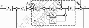
Fig. 1 Modified cascade control structure

In the nominal case, P_2m is perfect model of the intermediate process. From Fig. 1, it can be determined that the transfer functions are in the form of

                           (1)

                         (2)

            (3)

 　　　        (4)

It can be seen from Eqs. (1)-(4) that the performance of set-point and load disturbance rejection response in both loops are decoupled completely, and it requires the design of three controllers C₁(s), C₂(s) and C₃(s). In process industries, usually, the secondary process dynamics is stable in nature and the dynamics of the primary process is stable/integrating/unstable based on the dynamics of the process in cascade control loops [3]. Without loss of generality, the classes of processes with time delay can be represented by the following transfer function models:

1) First-order plus time delay process (FOPDT)

                         (5)

                        (6)

2) Unstable first-order plus time delay process (UFOPDT)

                         (7)

                        (8)

3) Integrating plus first-order plus time delay process (IPFOPDT)

                       (9)

                       (10)

where P₁(s) denotes the primary process and P₂(s) denotes the intermediate stable process.

2.1 Set-point tracking controller C₂(s) of inner loop

In the proposed control program, C₂(s) is used for the purpose of reducing the deviation and realizing the set-point tracking. According to the IMC design method, it can be easily got by

                   (11)

where λ_c2 is the adjustable parameter. It can be seen from Eq. (1) that in the nominal case, the set-point tracking control is open-loop control, and the set-point transfer function can be got:

                     (12)

The tuning of the adjustable parameter λ_c2 aims at a trade-off between the nominal performance of the set-point tracking controller C₂(s) and its corresponding actuator. Usually, λ_c2 can be chosen equal to the inner-loop time delay, in order to have a faster secondary loop dynamics. It can be chosen as one-half the time delay of the inner loop.

2.2 Load disturbance rejection controller C₃(s) of inner loop

Using Eq. (3), we obtain the closed-loop complementary sensitivity function as

                 (13)

By comparing Eq. (13) and Eq. (1), it can be seen that they have the identical form. So using the same method with C₂(s) can devise the disturbance rejection controller C₃(s):

                         (14)

where λ_c3 is the adjustable parameter for meeting the system operation requirement for rejecting load disturbance. It can be seen form Eq. (12), Eq. (3) and Eq. (13) that in the second loop, the response of set-point tracking and the load disturbance rejection are decoupled completely, and we can adjust the performance of disturbance rejection using the adjustable parameter. Decreasing λ_c3 improves the disturbance rejection performance of the closed-loop but decays its robust stability; on the contrary, increasing λ_c3 tends to strengthen the robust stability of the closed-loop but degrades its disturbance rejection performance.

2.3 Designing outer loop controller C₁(s)

The inner closed-loop transfer function can be got from Eq. (12), and the overall plant transfer function for the outer-loop is

            (15)

1) For the FOPTD process, the overall plant transfer function for the outer loop is

  (16)

According to the relationship between the internal mode control and unit feedback control, minimized sensitivity method is adopted to design the controller [18]. Suppose that

                   (17)

Hence, the sensitivity function of the closed-loop between the process input and output for the load disturbance rejection is obtained as

                          (18)

Define the optimal performance criteria to be   min||W(s)S(s)||_∞, where W(s) is the weighting function. Usually, in process control, W(s) can be selected as 1/s. According to the H_∞ control theory and the well-known maximum modulus theorem, it can be got

       (19)

Approximate the time delay by a first-order Taylor series, . Therefore, the optimal Q(s) is obtained as

            (20)

where λ_c1 is adjustable parameter. Then, substituting   Eq. (20) into Eq. (17) and approximating the time delay by a first-order Taylor series can obtain the controller C₁(s):

          (21)

Mathematical Maclaurin expansion series is utilized to copy out the controller C₁(s) in Eq. (21). Let C₁(s)=M(s)/s, and it follows that

        (22)

Obviously, the first three terms of the above Maclaurin expansion constitute exactly a standard PID controller in form of

                      (23)

where k_c=f ′(0), T_I=f ′(0)/f(0) and T_D=f ′′(0)/2f ′(0).

For UFOPTD process, there is no need to add the filter F₁(s). By substituting Eqs. (21) and (12) into    Eq. (3), the setpoint response transfer function of outer-loop is obtained in form of

                   (24)

Obviously, the setpoint transfer function is stable. When λ_c1  is tuned to be zero, it comes to the ideal case . It can be seen that there is no overshoot in the nominal setpoint response and the system response can be tuned by the single adjustable parameter λ_c1. Based on many simulation studies, it is observed that the starting values of the tuning parameter λ_c1 can be set equal to the corresponding overall primary process time delay. If the performance with the value is acceptable, then the value can be taken as the final value; if not, the parameter should be tuned again, and it is recommended to be in the range from 0.5(θ₁+θ₂) to 1.2(θ₁+θ₂).

2) For the UFOPTD process, the overall plant transfer function for the outer loop is

(25)

Accordingly, the setpoint tracking controller C₁(s) can be derived by a similar design procedure as above, that is

    (26)

where Analogously, the executable  can be obtained in form of PID by using Eqs. (22) and (23).

Different from the FOPTD process, the setpoint tracking performance of controller C₁(s) for UFOPTD process is not satisfactory. So, in order to improve the setpoint tracking performance and reduce the overshoot, a setpoint filter is designed:

                      (27)

3) Analogously, as for the IPFOPTD process, the overall plant transfer function for the outer loop is

(28)

Accordingly, the setpoint tracking controller C₁(s) can be derived by a similar design procedure as above, that is

    (29)

where In the same way, the executable C₁(s) can be obtained in form of PID by using Eqs.(22) and (23), and the setpoint filter is designed:

                      (30)

As for the UFOPTD and IPFOPTD processes, theoretically, the setpoint filter is F₁(s)= . But because the controller C₁(s) is obtained using the approximate method, the filter should be adjusted near a in practice to obtain the excellent setpoint tracking performance.

3 System robust stability analysis

In industrial and chemical practice, frequently encountered process uncertainties are the perturbation of the process parameters, the actuator output uncertainties, and the measurement uncertainties of the process sensors. A practical way to identify the closed-loop system robust stability in the presence of the above-mentioned process uncertainties is to lump multiple sources of uncertainty into a multiplicative form [11]. To evaluate the robustness of the system, the uncertainty structure of the cascade system is shown in Fig. 2.

To analyze the robustness of the closed loop system with the plant uncertainty, we put the system into an equivalent M-Δ structure, as shown in Fig. 3.

M is the transfer matrix from signals d_2i, d_2o, d_1i, d_1o to y₂, u₂, y₁, u₁:

where According to the small μ theorem, the closed loop system is robustly stable for all ||Δ||_∞≤γ if and only if μ_Δ(M)<1/γ [19]. The smaller the μ_Δ(M) is, the more robust the closed loop system is. In the same way, we can analyze the uncertain structure robustness of the inner-loop and outer-loop separately. For example, if uncertainty is only presented in the inner-loop, just upper 2×2 block of the transfer matrix M is considered, and lower 2×2 block of the transfer matrix M is considered for the outer-loop. Matlab robust control toolbox can be used to calibrate μ_Δ(M) [20].

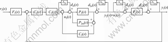
Fig. 2 Uncertainty structure of cascade system

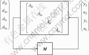
Fig. 3 M-Δ structure

4 Simulation examples

4.1 Example 1

Consider the open-loop stable cascade control system studied by IBRAHIM et al [7]:

 

In the method, a modified cascade control scheme combined with Smith predictor was proposed, and it had already been demonstrated that its superiority was better than many other previous approaches. The three controllers were respectively G_c1=0.5(1+1/0.25s),  and  In the proposed method, take  and obtain the controllers in form of    Because ,  is got. By adding a unit step change to the set point input at t=0 s, an inverse unit step change of load disturbance to the intermediate process output at t=400 s, and an inverse step change of load disturbance with magnitude of 0.1 to the primary process output at t=600 s, the simulation results are obtained, as shown in Fig. 4.

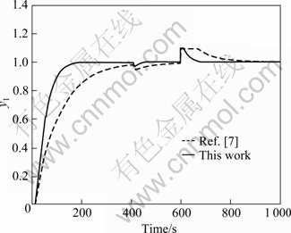
Fig. 4 Nominal system responses of Example 1

Now suppose that there exists 50% error for estimating the process time delay and the time constant of the primary process model, such that both of them are actually 50% larger, that is, . The perturbed system response is provided in Fig. 5.

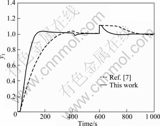
Fig. 5 Perturbed system responses for Example 1 (Parameters of primary controllers changed)

Suppose that there exists 50% error for estimating the process time delay and the time constant of the secondary process model, such that both of them are actually 50% larger, that is, . The system response is provided in Fig. 6.

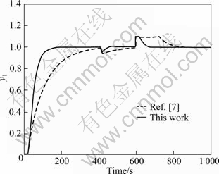
Fig. 6 Perturbed system responses for Example 1 (Parameters of secondary controllers changed)

It can be seen from the simulation results that the proposed method gives slightly better performances for the open-loop stable process.

4.2 Example 2

Consider a chemical CSTR studied by LIU et al [11], of which the intermediate stable process and the primary unstable process are respectively identified as

,     

In Ref. [11], a three degree-of-freedom control structure was proposed for unstable cascade process, of which four controllers are C(s)=(400s²+ , and  In the proposed method, take   and obtain the controllers in form of and  .

By adding a unit step change to the set point   input at t=0 s, an inverse step change of load disturbance with magnitude of 0.5 to the intermediate process output at t=200 s, and an inverse step change of load disturbance with magnitude of 0.1 to the primary process output at t=400 s, the simulation results are obtained, as shown in Fig. 7. It is seen that the proposed controller leads to obviously improved load disturbance performance. Figure 8 shows the corresponding   control action response of controller C₁(s), namely the output of y₂(s). It can be seen that the control action variation for the proposed method is comparatively smooth.

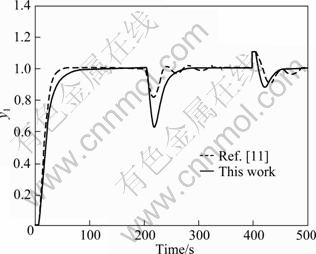
Fig. 7 Nominal system responses of Example 2

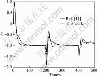
Fig. 8 Nominal system responses of inner-loop of Example 2

Now suppose that there exists 50% error for estimating the process time delay and the time constant of the primary process model, such that both of them are actually 50% larger, that is . The perturbed system response is provided in Fig. 9. It can be observed that the proposed method gives better control performance comparatively. Suppose that there exists 30% error for estimating the process time delay and the time constant of the secondary process model, such that both of them are actually 30% larger, that is,The system response is provided in Fig. 10. It is seen that better system response stability is obtained by the proposed cascade control method.

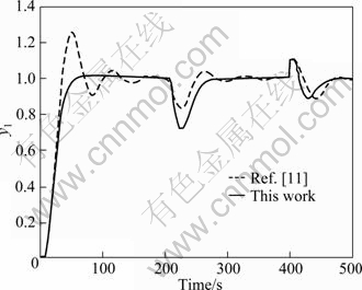
Fig. 9 Perturbed system responses for Example 2 (Parameters of primary controllers changed)

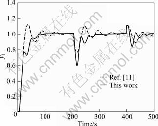
Fig. 10 Perturbed system responses for Example 2 (Parameters of secondary controllers changed)

4.3 Example 3

An example studied by UMA et al [3] is considered. The cascade process is considered as

 

According to the proposed method, take , ,, and obtain the controllers in form of ,. For the process, a filter to the derivative term in PID controller is added, and then  and C₁(s)= are got.

With these controllers settings, simulation studies are carried out by giving a unit step input in the set point at t=0 s, negative disturbance of 0.1 in the inner loop at t=80 s and negative disturbance of magnitude 0.1 in d₁₀ at t=160 s. The corresponding system response is shown in Fig. 11, where the solid line denotes the nominal system response, the dash dot line denotes the perturbed system response of , and the dot line denotes the perturbed system response of , while the intermediate process P₂(s) remains unchanged.

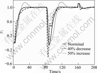
Fig. 11 System responses of parameters changed in P₁ for Example 3

To illustrate the robust stability of the system to the parameters changed in intermediate process P₂(s), uncertainty of 50% in t₂, θ₂ and -50% in t₂, θ₂ are considered. The corresponding response is shown in  Fig. 12, where the solid line denotes the nominal system

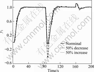
Fig. 12 System responses of parameters changed in P₂ for Example 3

response, the dash dot line denotes the perturbed system response of , and the dot line denotes the perturbed system response of  , while the primary process t₂, P₁(s) remains unchanged.

5 Conclusions

1) Two-degree-of-freedom control scheme both in primary loop and secondary loop based on internal mode control is proposed for cascade processes with time delay.

2) The two controllers in the inner-loop are designed using IMC procedure, and can be monotonically tuned by a single adjustable parameter.

3) The controller in the primary loop is designed using an optimization method of H_∞ performance criterion, and constitutes in PID form.

4) The simulation results show that the proposed method can achieve better control performance in both nominal case and model mismatch case than other methods. What’s more, the proposed method can be used for all kinds of cascade processes.

References

[1] SONG Si-hai, CAI Wen-jian, WANG Ya-gang. Auto-tuning of cascade control systems [J]. ISA Transactions, 2003, 42(1): 63-72.

[2] UTKAL M, SOMANATH M. On-line identification of cascade control systems based on half limit cycle data [J]. ISA Transactions, 2011, 5(3): 473-478.

[3] UMA S, CHIDAMBARAM M, SESHAGIRI R A. Enhanced control of integrating cascade processes with time delays using modified Smith predictor [J]. Chemical Engineering Science, 2010, 65(3): 1065-1075.

[4] TAN K, LEE T H, FERDOUS R. Simultaneous online automatic tuning of cascade control for open loop stable processes [J]. ISA Transactions, 2000, 39 (2): 233-242.

[5] ALFARO V M, VILANOVA R, ARRIETA O. Two-degree-of- freedom PI/PID tuning approach for smooth control on cascade control systems [C]// 47th IEEE Conference on Decision and Control. Cancun, Mexico, 2008: 9-11.

[6] ALFARO V M, VILANOVA R, ARRIETA O. Robust tuning of two-degree-of-freedom (2-Dof) PI/PID based cascade control systems [J]. Journal of Process Control, 2009, 19(10): 1658-1670.

[7] IBRAHIM K, TAN N, DEREK P A. Improved cascade control structure for enhanced performance [J]. Journal of Process Control, 2007, 17(1): 3-16.

[8] LIU Tao, GU Dan-ying, ZHANG Wei-dong. Decoupling two-degree- of-freedom control strategy for cascade control systems [J]. Journal of Process Control, 2005, 15(2): 159-167.

[9] LIU Tao, ZHANG Wei-dong, GU Dan-ying. Analytical design for a class of open-loop unstable cascade control systems [J]. Journal of Control and Decision, 2004, 19(8): 872-876. (in Chinese)

[10] SARAF V, ZHAO F T, BEQUETTE B W. Relay autotuning of cascade-controlled open-loop unstable reactors [J]. Ind Eng Chem Res, 2003, 42(20): 4488-4494.

[11] LIU Tao, ZHANG Wei-dong, GU Dan-ying. IMC-based control strategy for open-loop unstable cascade processes [J]. Ind Eng Chem Res, 2005, 44(4): 900-909.

[12] LEE Y, SUNGOOL O, SUNWON P. Enhanced control with a general cascade control structure [J]. Ind Eng Chem Res, 2002, 41(11): 2679-2688.

[13] IBRAHIM K, DEREK P A. Use of smith predictor in the outer loop for cascade control of unstable and integrating processes [J]. Ind Eng Chem Res, 2008, 47(6): 1981-1987.

[14] DOLA G P, SOMANATH M. Modified smith predictor based cascade control of unstable time delay processes [J]. ISA Transactions, 2012, 51(1): 95-104.

[15] DOLA G P, SOMANATH M. An improved parallel cascade control structure for processed with time delay [J]. Journal of Process Control, 2012, 49(6): 546-558.

[16] RAO A S, SEETHALADEVI S, CHIDAMBARAM M. Enhancing the performance of parallel cascade control using Smith predictor [J]. ISA Transactions, 2009, 48(2): 220-227.

[17] LEE Y, SKLIAR M, LEE.M Analytical method of PID controller design for parallel cascade control [J]. Journal of Process Control, 2006, 16(8): 809-818.

[18] ZHANG Wei-dong, XU Xiao-ming, SUN You-xian. Quantitative performance design for integrating processes with time delay [J]. Automatica, 1999, 35(4): 719-723.

[19] ZHOU K, DOYLE J C. Essentials of robust control [M]. Upper Saddle River: Pentice Hall, 1998: 129-150.

[20] RICHARD Y C, MICHAEL G S. Robust control toolbox user’ guide [M]. 3rd Edition, Natick, MA: The MathWorks, Inc, 1998: 26-38.

(Edited by YANG Bing)

Foundation item: Project(J11LG02) supported by the Science and Technology Funds of Education Department of Shandong Province, China

Received date: 2011-07-26; Accepted date: 2011-11-14

Corresponding author: YIN Cheng-qiang, Associate Professor, PhD; Tel: +86-635-8239877; E-mail: shtjycq@163.com