J. Cent. South Univ. Technol. (2011) 18: 773-781
DOI: 10.1007/s11771-011-0762-y
Unbiased parameter estimation of continuous-time system based on modulating functions with input and output white noises
HE Shang-hong(贺尚红), LI Xu-yu(李旭宇)
School of Automobile and Mechanical Engineering, Changsha University of Science and Technology,
Changsha 410114, China
? Central South University Press and Springer-Verlag Berlin Heidelberg 2011
Abstract: An efficient unbiased estimation method is proposed for the direct identification of linear continuous-time system with noisy input and output measurements. Using the Gaussian modulating filters, by numerical integration, an equivalent discrete identification model which is parameterized with continuous-time model parameters is developed, and the parameters can be estimated by the least-squares (LS) algorithm. Even with white noises in input and output measurement data, the LS estimate is biased, and the bias is determined by the variances of noises. According to the asymptotic analysis, the relationship between bias and noise variances is derived. One equation relating to the measurement noise variances is derived through the analysis of the LS errors. Increasing the degree of denominator of the system transfer function by one, an extended model is constructed. By comparing the true value and LS estimates of the parameters between original and extended model, another equation with input and output noise variances is formulated. So, the noise variances are resolved by the set of equations, the LS bias is eliminated and the unbiased estimates of system parameters are obtained. A simulation example by comparing the standard LS with bias eliminating LS algorithm indicates that the proposed algorithm is an efficient method with noisy input and output measurements.
Key words: continuous-time system; unbiased parameter; modulating functions; noise
1 Introduction
The parameter estimation methods for discrete-time (DT) model based on sampled data have been fairly well developed [1]. But, most real dynamical systems in the physical system are normally formulated in the continuous-time (CT) domain, such as differential equations, and partially differential equations. So, the CT model is the most natural representation of physical system and has more merits and significance than the discrete-time model [2-3].
There are two general methods for the parameter estimation of continuous-time systems. The first is the indirect method, in which the system is approximated as a DT model, and the parameters are estimated in DT domain and then transformed to CT domain. This approach has the advantage of using all of the estimation methods for DT models. But, the conventional DT methods are not in harmony with the CT domain even with reduced sampling period. In some cases, they do not converge to the results corresponding to the original CT model.
Another method is the direct approach which has been received more and more attention in recent years. The bottle-neck of direct method is the difficulty of measurement of derivative terms in the CT model. The digital approximation of derivatives of input-output signals may give rise to the accentuation of measurement noises. So, in direct method, the CT system parameters are estimated through processing the original differential equations, often by the use of filters or other operators [2].
Many approaches are available for the direct identification of the CT models. The modulating function method is an efficient approach because it not only avoids the approximation of time derivatives of measured signals, but also does not require the knowledge of the initial conditions [3]. By multiplying modulating functions with both sides of differential equation and applying integral over a period of time, the original differential equations can be converted into a set of algebraic equations. Using multiple integral rule and digital integral approximation, the equivalent algebraic equation which is convenient for computer calculation can be obtained. So, the parameters can be estimated with the standard least-squares (LS) algorithms [4-5]. Recently, the modulating function method is applied to the parameter estimation of automatic gauge control system of a steel rolling mill [5-6].
The consistent and unbiased estimation method is the main task of system identification during the last two decades. As to DT estimation problem, in which the measurement of the system output is corrupted by noise while the input is noise-free, there are many methods to get unbiased estimation, such as instrumental variable method, augmented LS, and generalised LS [1]. In practical circumstances, the system input is also contaminated by noise. System identification using measurements of both noisy output and noisy input data turns out to be a much more formidable problem. FENG and ZHENG [7] proposed a famous bias-eliminated LS (BELS) method, in which a designed filter is inserted into the identified system so that the resulting system has some known zeros. This method can be used for eliminating the noise-induced bias in LS estimates. The difficulty of this method is the optimal choice of the filter.
It has been proved that even the input and output measurement noises are white noises, the estimates are biased and the bias is determined by the noise variances [8]. The asymptotic analysis of the mean error can provide one of the two equations needed for determining the variances of the input and output noises. By increasing the denominator of the transfer function by one dimension, the second equation explicitly related to the variances is obtained. Solving the set of these two equations will yield the estimates of the measurement noise variances, so the unbiased estimation can be obtained by bias elimination [8-9].
As to the modulating function method for the CT system identification, because of digital modulating integral of both input and output noises, the disturbance term of the equivalent identified model is very complicated. So, few researches about the unbiasedness of the digital modulating functions method are reported. PREISIG and RIPPIN [10] investigated the filtering characteristics of spline-type modulating function, and analyzed the influence of the order, time characteristic constant and shifted time interval on the identification accuracy. In Refs.[4-5], modulating functions were constructed by dilating the Gaussian based function. The relationship between the accuracy of identification and the dilating factor of modulating functions was investigated. It has been conformed that, to improve the accuracy of the parameter estimates, the dilating factor should be chosen so that the frequency bandwidth of modulating filter matches the frequency bandwidth of the system as closely as possible.
Further research about modulating function method indicates that, like LS estimator of DT model, the LS estimator is biased even with white measurement output noise, and the bias is determined by the variance of output noise. The unbiased estimator can be got through the elimination of output noise induced bias [11].
The content of the present work is the development of bias eliminating method of Ref.[11]. Using the thoughts of Refs.[8-9], taking account of both input and output measurement white noises, the relationship between estimation bias and noise variances is derived, and two algebraic equations about input and output noise variances are acquired. By solving the set of equations, the noise variance estimates are got, and the unbiased estimation is implemented through bias elimination.
2 Principle of modulating function method
Consider a single-input and single-output (SISO) continuous-time system described by the linear differential equation model:
 (1)
(1)
where r(t) is the input signal and x(t) the output response to r(t); t is the time; n and m are the orders of model, n≥m; ai and bi are parameters of the model.
Assume modulating function f(t), which satisfies
 (2)
(2)
and the i-th derivative of f(t),  (i=1, 2, …, n) exists, and
 (3)
(3)
Both sides of Eq.(1) are multiplied by f(t) and integrated over the time interval [0, T], and are repeatedly integrated by parts. Using Eqs.(2) and (3), the equivalent modulating integral equation is got:

 (4)
(4)
Compared with Eq.(1), the derivatives of signal r(t) and x(t) which lead to the noisy-accentuating are avoided.
Dilating the Gaussian function defined by 
exp(-t2/2), by scaling factor a, the modulating function and their derivatives can be got:
 (5)
(5)
 (6)
(6)
 (7)
(7)
…
The characteristic time T satisfies: T≈8a,  ≈0,
≈0,  ≈0. So, T can be adjusted with the scaling factor a.
Assume now that the window interval of modulating function f(t) is T=nf?ts, where ?ts is the sampling time interval, and nf +1 is the sampling number of modulating function at [0, T]. The i-th derivative, f(i)(t), is represented as {f(i)(j?ts)} (j=0, 1, …, nf). For convenience, f(i)(j?ts) is replaced by f(i)(j), and also r(k), x(k), etc will be used in the same way.
With trapezoidal integral rule, if the truncation error is ignored, the modulating integral of the i-th derivative of z(t) over the time interval [t-T, t] is

 (8)
(8)
where
 (9)
(9)
 (10)
(10)
Introducing a delay operator q-j, i.e. q-jz(t)= z(t-jΔts), q0z(t)=z(t), Eq.(8) can be approximated as
 (11)
(11)
where
 (12)
(12)
Fi(q-1)z(t) is the modulating integral of the i-th derivative of z(t) over the time interval nfΔts at the beginning time point t. Apply polynomial Fi(q-1) to time series {z(k)}, modulating series {Fi(q-1)z(k)} are generated according to the following rule: the first signal data correspond to the beginning point of the first modulating window. At next modulating integral, the data window with fixed size T moves forward a time step Δts.
As to Eq.(4), substituting integral interval [kΔts- nfΔts, kΔts] for [0, T], the equivalent form of original differential model is represented as
 (13)
(13)
In the actual situation, the input and output are polluted by the measurement disturbance noises. So, the actual input and output are: u(k)=r(k)+vu(k) and y(k)= x(k)+vy(k).
Equation (13) becomes
 (14)
(14)
where is the vector of the parameters;
 [
[
 ]T;
]T;
 =[F0(q-1)u(k) F1(q-1)u(k) … Fm(q-1)u(k)]T;
 =[-F1(q-1)y(k) … -Fn(q-1)y(k)]T.
e(k)==C(q-1)vy(k)+D(q-1)vu(k) (15)
where
 (16)
(16)
 (17)
(17)
From Eq.(14), the LS estimate, θLS, is obtained as
 (18)
(18)
3 Principle of bias elimination
By substituting Eq.(14) into Eq.(18), the following equation will be obtained [11]:
θLS(l)=θ+Δθ=θ+Rψψ(l)-1Rψe(l) (19)
where
 (20)
(20)
 (21)
(21)
According to the asymptotic characteristics of standard LS estimator θLS(l), there is
 w.p.1 (22)
where Δθ is the estimate bias as
 (23)
(23)
 (24)
(24)
 (25)
(25)
Rψψ is the autocorrelation matrix of ψ, and Rψe is the cross correlation vector of ψ and e.
Supposing that the input and output measurement noise vu(k) and vy(k) is a zero-mean identically and independently distributed Gaussian sequence with variance  and
and  respectively, there are
 (26)
(26)
 (27)
(27)
 (28)
(28)
where
 (i=0, 1, …, m)
 (i=1, …, n)
From Eq.(28),


 (29)
(29)
where
 (30)
(30)
So,
 (31)
(31)
where In, Im+1 are the unit matrixes with dimension n and m+1 respectively; θ0 is the true parameter vector of model.
The unbiased estimate of  is
is
 (32a)
(32a)
Equation (32a) reveals that θLS is biased due to the presence of measurement noises, and the asymptotic bias clearly depends upon the noise variances and . Therefore, once and are known, the bias can be eliminated from θLS to get unbiased estimation. Because the variances and are unknown, , and model parameters must be estimated simultaneously. So, Eq.(32a) should be represented by
 (32b)
(32b)
4 Estimation of variances
Define LS error as
 (33)
(33)
Substituting Eq.(18) into Eq.(33), there is

 (34)
(34)
Substitute Eq.(14) into Eq.(33) to get
 (35)
(35)
From Eqs.(34) and (35), the average value  is
is

 =
=
 =
=

 (36)
(36)
From Eqs.(15) and (26), there is
E[e(i)2]=E{ }+E{
}+E{ }+
}+
2E{[ ][
][ ]}=
]}=
 (37)
(37)
From Eqs.(29), (37) and (36), there is
E[ (i)2]=

-H(θ0)Tdiag(Im+1, In+1)(θ0- (l))+
(l))+
 (38)
(38)
Let δθ=θ0- (l)=[
(l)=[
 ]T
]T
where
 =
= -
- (l)
(l)
 =
= -
- (l)
(l)
From Eq.(29), there is
-H( )Tdiag(Im+1,In)(-
 (l)) =
-[ ,
,  ] (39)
So, Eq.(38) is converted as
E[(i)2]= +
+ (40)
(40)
where
 (41)
(41)
The estimate of Eq.(40) is
 (42)
(42)


 and
and  are the estimates of θa0, θb0, and , respectively.
Equation (42) is an algebraic equation about and . Another equation must be acquired to get and .
To get another equation about and , an augmented transfer function is introduced:
 (43)
(43)
where 
Define  which is the parameter vector of augmented system Eq.(43).
If the augmented system is equivalent to the original system, the parameters of two systems should be satisfied as
 (44)
(44)
Like above processing procedure, we can get
F0(q-1)y(k) = (k)T
(k)T +
+ (45)
(45)
where
 (46)
(46)
 (47)
(47)
 (j=0, 1, …, nf) (48)
The LS estimate of is
 (49)
(49)
where
 (50)
(50)
 F0(q-1)y(k)=[W(l)T w(l)]T (51)
 F0(q-1)y(k) (52)
 (53)
(53)
The true value of is
 (54)
(54)
Just like Eq.(31), and considering (an+1)0=0, there is

 (55)
(55)
where
 [
[

 (56)
(56)
 (57)
(57)
 is expressed as
 (58)
(58)
where
 (59)
(59)
 (60)
(60)
According to the matrix inversion rule [1], there is

 (61)
(61)
where
 (62)
(62)
Substituting Eqs.(61) and (51) into Eq.(49), (an+1)LS becomes
 (63)
(63)
Let [Lu Ly], where
 Substituting Eqs.(61), (62), (44) and (55) into Eq.(54), it yields
 =
= -
-


 (64)
(64)
So,


 (65)
(65)
From Eqs.(63) and (65), there is
[Lu ]+[Ly
]+[Ly +
+ ]=
]=
 (66)
(66)
The estimate of Eq.(66) is
[Lu ]+[Ly
]+[Ly +
+ ]
] =
=
 (67)
(67)
Equations (42) and (67) constitute a set of equations. Resolving the set of equations, and can be solved obviously.
From above derivation, θLS,  and should be estimated via the iterative procedure.
5 Recursive estimation algorithm
With the preparation for recursive procedure, pj (j=0, 1, …, nf) and  (i=0, 1, …, n+1; j=0, 1, …, nf) are calculated.
Set initial estimates: 
 and PLS(0).
Let k=1, and implement the following recursive procedure:
0(k)=LS(k)+
kP(k)diag[(k)Im+1,(k)In]H(0(k-1)) (68)
LS(k)=LS(k-1)+L(k)ε(k) (69)
L(k)= (70)
(70)
P(k)=[I-L(k) (71)
(71)
ε(k)=F0(q-1)y(k)- (72)
(72)
 =
=

 (73)
(73)
where
ρ(k)= (74)
(74)
f(k)= F0(q-1)y(i) (75)
-kρ(k)TP(k)=[Lu(k) Ly(k)] (76)
 (77)
(77)
 (78)
(78)
 (79)
(79)
 (80)
(80)
 (81)
(81)
and PLS(0) can be determined by the following steps:
1) Take standard estimates as the initial values
 (82)
(82)
 (83)
(83)
2) Estimate  with standard recursive LS algorithm for rn step, take the final value as the initial value:
  The initial estimates of standard recursive LS are: with any value, PLS(0)=γIn×n, where γ is a enough real value, In×n is unit matrix with dimension n.
6 Simulation example
Consider a second-order system described by G(s)= (b1s+b0)/(s2+a1s+a0) with b0=1.25, b1=0, a0=0.7, a1=0.25 and input u(t) chosen as inverse repeated pseudo-random binary sequence (PRBS) superimposed by zero-mean Gaussian sequence with a standard deviation of 0.1. The periodic length of PRBS is N=31 and the pulse period time is 20 ms.
The measurement noise v(k), which is input noise vu(k) or output noise vy(k), is a zero-mean identically and independently distributed Gaussian sequence. Its variance is adjusted to obtain the desired ratio of noise to signal (N/S) defined by
 (84)
(84)
where σv and σx represent the standard deviations of noise ν and signal x, respectively. In the example, N/S ratios of input and output are 10% and 40%, respectively.
The sampling time Δts is 20 ms, and the signal lasting length is 61.44 s. The modulating window width T is 1 s or 2 s. Execute the standard recursive least- squares (RLS) for 1 000 time step, then turn to bias eliminating RLS (BERLS). Make the recursive results of 3 000 time steps as the final results. The initial value for standard RLS is  PLS(0)=γI4×4, γ=108.
For comparing the standard RLS and BERLS, define the normalized error of LS estimates as
 (85)
(85)
where N is the number of independent experiments (N=50), θ0 and are the true and estimated parameters, respectively. The input and output measurement noises are generated independently every time, but the noise-free input and output data are kept the same.
In Refs.[4-5], it was proved that when the frequency bandwidth of modulating integral filter matches the frequency bandwidth of the system as closely as possible, accurate estimates can be got even with high N/S ratio.
Table 1 lists the comparison result between RLS and BERLS with T=1 s and T=2 s. It can be found that when T=2 s, the frequency bandwidth of the modulating integral filter is close to the given system [4-5]. So, when T=2 s, the BERLS has no evident predominance over RLS.
On the contrary, if T is taken to be less than 2 s, the frequency bandwidth of the modulating integral filter is wider than that of the given system [4-5]. When T=1 s, the frequency bandwidth of the modulating integral filter is about two times that of the given system. The normalized errors of RLS and BERLS are 24.6% and 9.43%, respectively. This is because the measurement noises with frequency bandwidth beyond that of the given system are not filtered efficiently. So, the LS estimates become worse, and the BERLS has evident superiority over RLS.
Figure 1 illustrates the process of RLS and BERLS contrastively with unmatched modulating functions (T= 1 s). It is proved that the RLS converges to biased value from true parameters. When RLS turns to BERLS at the recursive step of 1 000, estimates converge closely to true values rapidly because of the bias elimination. b0, a1 and a2 of BERLS are obviously accurate than those of RLS, but b1 has not been improved. Actually, in this example, b1 values of RLS and BERLS are very close to true value of 0. The coordinate range of b1 in Fig.1 is [-0.1 0.1], which amplifies the difference of two methods.
Figure 2 shows the recursive estimation process of noise variances, indicating the validity of the estimation method of noise variances.
Table 1 Comparison between RLS and BERLS
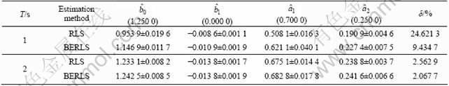
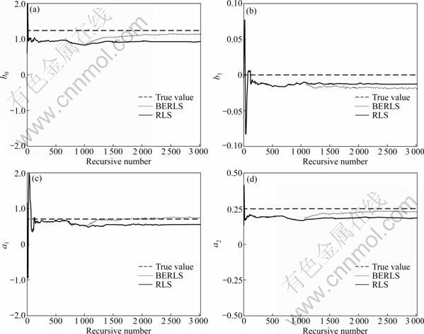
Fig.1 Comparison of process of RLS and BERLS with unmatched modulating functions (T=1 s): (a) b0; (b) b1; (c) a1; (d) a2
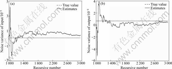
Fig.2 Estimates of noise variances: (a) Input noise variance; (b) Output noise variance
7 Conclusions
1) With input and output white noises, the LS estimates of continuous time system using the modulating functions method are biased. The bias is determined by the noise variances.
2) By the asymptotic analysis of LS estimates, one algebraic equation relating the measurement noise variances and the LS errors is derived. The degree of denominator of the original system transfer function is increased by one to construct an extended model. Another equation with noise variances is formulated by comparing the true value and LS estimates between original and extended model. The noise variances are resolved by the set of equations. The unbiased estimates of the continuous time system can be acquired recursively through the bias elimination.
3) The simulation example indicates that, when the bandwidth of modulating filters does not match that of the identified system, the RLS cannot obtain accurate estimates, but the BERLS can improve the accuracy efficiently. So, when we have little knowledge about the frequency bandwidth of the identified system, we should implement the BERLS to get unbiased estimates.
References
[1] FANG Cheng-zhi, XIAO De-yun. Process identification [M]. Beijing: Tsinghua University Press, 1989: 1-562.
[2] HNBEHAUEN H, RAO G P. A review of identification in continuous-time systems [J]. Annual Review in Control, 1998, 22: 145-171.
[3] BALESTRINO A, LANDI A, SANI L. Parameter identification of continuous systems with multiple-input time delays via modulating functions [J]. IEE Proceedings Part D: Control Theory and Applications, 2000, 147(1): 19-27.
[4] HE Shang-hong, ZHONG Jue. Identification of linear continuous- time system using wavelet modulating filters [J]. Journal of Systems Engineering and Electronics, 2004, 15(3): 270-277.
[5] HE Shang-hong, ZHONG Jue. Parameter estimation of linear continuous-time dynamic system using modulating functions method [J]. Chinese Journal of Mechanical Engineering, 2003, 39(12): 129-134.
[6] HE Shang-hong, ZHONG Jue. Modeling and identification of HAGC system of a temper rolling mill [J]. Journal of Central South University of Technology, 2005, 12(6): 699-704.
[7] FENG C B, ZHENG W X. Robust identification of stochastic linear systems with correlated noise [J]. IEE Proceedings Part D: Control Theory and Applications, 1991, 138(5): 484-492.
[8] ZHENG W X. Transfer function estimation from noise input and output data [J]. Internal Journal of Adaptive Control & Signal Processing, 1998, 12(4): 365-380.
[9] ZHENG W X. Noisy input-output system identification using the least-squares based algorithms [C]// Proceedings of the 37th IEEE Conference on Decision & Control. Tampa, 1998: 725-730.
[10] PREISIG H A, RIPPIN D W T. Theory and application of the modulating function method (Ⅱ): Algebraic representation of Maletinsky’s spline-type modulating functions [J]. Computer Chem Engng, 1993, 17(1): 17-28.
[11] HE Shang-hong, ZHONG Jue. Bias compensating direct identification of continuous time system with noisy output data [C]// Proceedings of the 6th World Congress on Intelligent Control and Automation. Dalian, 2006: 1421-1425.
(Edited by YANG Bing)
Foundation item: Project(50875028) supported by the National Natural Science Foundation of China
Received date: 2009-09-14; Accepted date: 2010-03-25
Corresponding author: HE Shang-hong, Professor, PhD; Tel: +86-731-85258627; E-mail: heshh@csust.cn

