J. Cent. South Univ. Technol. (2008) 15(s1): 057-060

DOI: 10.1007/s11771-008-314-2

New algorithm applied to vibration equations of time-varying system

CHEN Rui-lin(陈锐林)^{1, 2}, ZENG Qing-yuan(曾庆元)¹, ZHANG Jun-yan(张俊彦)²

(1. School of Architectural and Civil Engineering, Central South University, Changsha 410075, China;

2. College of Civil Engineering and Mechanics, Xiangtan University, Xiangtan 411105, China)

Abstract: Vibration equations of time-varying system are transformed to the form which is suitable to precise integration algorithm. Precision analysis and computation efficiency of new algorithm are implemented. The following conclusions can be got. Choosing matrixes M, G and K is certainly flexible. We can place left side of nonlinear terms of vibration equations of time-varying system into right side of equations in precise integration algorithms. The key of transformation from vibration equations of time-varying system to first order differential equations is to form matrix H, which should be assured to be nonsingular. With suitable disposal, precision and computation efficiency of precise integration algorithms are greatly larger than those of general methods.

Key words: time-varying system; vibration analysis; precise integration algorithm

1 Introduction

Vibration equation of time-varying system^[1-2] is:

              (1)

where  M(t), G(t) and K(t) are matrices of mass, damp and stiffness, respectively, which are the functions of time. q(t) and F(t) are the vectors of displacement and force, seperately. (?) denotes the derivative to time.

The solutions of vibration equations of time-varying system are mainly involved of methods of direct numerical integral. The traditional methods of direct numerical integral include two categories, i.e. implicit and explicit methods. Implicit methods consist of newmark method, Wilson-θ method and Houbolt method, etc. Generally speaking, numerical stability of implicit methods is better than that of explicit methods, but implicit methods need to compute matrixs M, C and K in every time step, which causes difficulties in vibration analysis of multi-demension time-varying system, such as vehicle-bridge system and train-track system. Its calculation workload is very astonishing.

Commonly used explicit methods include four rank Runge-Kutta method^[3] and centre difference method. The calculation efficiency of explicit methods is higher, which is at cost of loss or decrease of accuracy and stability. ZHAI^[4-5] put forward a type of new explicit numerical integral method and a type of new estimate- correct integral method, which raise greatly calculation efficiency.

However, it is essential that a long period calculation is carried on for vibration analysis of multi-demension time-varying system in small time step. So when above-mentioned methods are applied to calculation, numerical dissipation is inevitable and everything is probably completely changed as a result.

This work puts forward a new solution. Vibration equations of multi-demension time-varying system are redirected to first order differential equations and solved by applying precise integration algorithms.

2 Precise integration algorithms^[6-8]

The problems of precise integration algorithms are as follows:

                                  (2)

                            (3)

where  p is the dual vector of q.

If H is Hamilton matrix, then it must satisfy JHJ= H^T.

                            (4)

where  I_n is unit matrix.

2.1 Precise integration algorithms of homogeneous equations

Firstly, we should solve homogeneous equations

                                     (5)

Its general solutions can be written as follows:

v=exp(Ht)?v₀                                 (6)

Now, time step is designated as τ, so the time moment is

t₀=0, t₁=τ, …, t_k=kτ, …                        (7)

And then we have

v(τ)=v₁=Tv₀, T=exp(Hτ)                        (8)

and

v₁=Tv₀, v₂=Tv₁, …, v_k+1=Tv_k, …                 (9)

Hence, the problem comes to the calculation of T, which should be very finely calculated.

We know

                   (10)

If m=2^N and N=20, then m=1 048 576, so Δt=τ/m is a very small time section.

Taylor series can be gotten

    (11)

As Δt is very small, the right side of above equation is very approximately equal to the left. Then the above equation can be written as

exp(H?Δt)≈I+T_a                            (12)

         (13)

where  T_a is a small variable. It is important that we should slove a T_a, not I+T_a. Because T_a is very small, it becomes its tail number and will lose almost accuracy in computer rounding operation.

In order to compute matrix T, we decompose

         (14)

The decomposition is done continuously for N times. so we can get the basic unit:

(I+T_b)(I+T_c)= I+T_b+T_c+T_bT_c                   (15)

Here, we take T_b, T_c as T_a, then calculation of T_a is recursive Procedure.

After we take the value of T_a, we can get T from the following formula:

T=I+T_a                                    (16)

2.2 Precise integration algorithms of non- homogeneous equations

We can think non-homogeneous terms are linear in time step (t_k, t_k+1), namely

                       (17)

where  r₀ and r₁ are designated vectors. On the supposition that Φ(t-t_k) is the solution of homogeneous equations, we have

                       (18)

So the solution of non-homogeneous equations can be given:

v=Φ(t-t_k)[v_k+H^-1(r₀+H^-1r₁)]-H^-1[r₀+H^-1r₁+r₁(t-t_k)] (19)

Though the analytical expression of Φ has not known yet, we have

Φ(t_k+1-t_k)=Φ(τ)=T                           (20)

Matrix T has been computed, then

v_k+1=T[v_k+H^-1(r₀+H^-1r₁)-H^-1[r₀+H^-1r₁+r₁?τ]]     (21a)

or

          (21b)

This is the formula of precise integration of non-homogeneous equations.

3 Control equations and its transformation

In Eqn.(1), we introduce variable substitution p, which is defined as

      (22)

So, Eqn.(1) can be written as

           (23)

Combining Eqns.(22) and (23), we can get the first order differential equation which is equivalent with the second order differential equation:

              (24)

where

              (25)

It should be noted that under the premise that computation efficiency is not decreased, how to choose matrixes M, G and K is certainly flexible. In consideration of simplifing, we take the simplest modal of single wheel attached to mass on the top of spring as example. In this modal, we take half of vehicle body as lumped mass and only consider vertical motion of body. Subtituting bogie mass into wheelset, we take vehicle as single dynamic system (Fig.1).

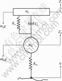
Fig.1 Model of single wheel

Vibration equation of vertical motion of vehicle body follows

      (26)

Vibration equation of vertical motion of wheelset follows

=-m_wg                         (27)

where  m_c is the vehicle body mass(half of vehicle); m_w is the wheelset mass; K_s and C_s are spring stiffness and damp coefficient of single dynamic system, respectively; K_w is the contact spring stiffness between wheelset and rail; and q is the displacement of the contact point between wheelset and rail.

Rewriting Eqns.(26) and (27) into equivalence form:

       (28)

       (29)

Rewriting Eqns.(28) and (29) in matrix form, we can get items in Eqn.(1). Here

We transform Eqn.(1) to the simple modal by Eqns.(22)-(25) and get Eqn.(24). This transform process and solution procedure can be implemented by computer programs conveniently.

4 Numerical implement

4.1 Computation process

Let us discuss the simplest modal of single wheel continuously.

In Eqn.(24), there is

where 

Then, the computer block diagram including transformation from the second order differential equation to the first order differential equation and precise integration algorithms of first order differential equation is carried on.

4.2 Analysis of precision and computation efficiency

Expanding Eqn.(11) must cause truncation error, and its value is about O(Δt⁵). Considering that Δt=τ/m≈ τ/10⁶ if N=20, we can conclude that truncation error corresponds to O((τ/10⁶)⁵). When algorithm 2N is carried on, the accumulation of error increases according to sum at most. Precision of other method, such as ZHAI’s new explicit numerical integral method, is about the same order as that of truncation error of Taylor series. i.e. O(τ^nth). Therefore, generally speaking, precision of new algorithm is greatly larger than that of general methods.

From Eqns.(12) and (13) we can see that we need to know matrix H and sub time step Δt in order to calculate T_a. Due to the transformation, we get matrix H. At the same time, sub time step can be taken by time step τ. Thus, calculating T is sequential process and its time cost will not be enhanced as the size of problem increases. Besides, because we deal with matrix H, and avoid computing matrixes M, G and K in every time step for vibration equations of time-varying system, this algorithm will greatly enhance the computation efficiency.

5 Conclusions

1) Choosing matrixes M, G and K is certainly flexible. We can place left side of nonlinear terms of vibration equations of time-varying system into right side of equations in precise integration algorithms.

2) Key of transformation from vibration equations of time-varying system to the first order differential equations is to form matrix H, which should be assured to be nonsingular.

3) After the above disposal is done, precision and computation efficiency of precise integration algorithms are greatly higher than those of general methods.

References

[1] ZENG Qing-yuan, GUO Xiang-rong. Theory of vibration analysis of railway-bridge time-varying system and its applications [M]. Beijing: China Railway Publishing House, 1999. (in Chinese)

[2] ZENG Qing-yuan, XIANG Jun, LOU Ping. A breakthrough in solving the problem of train derailment—The approach of random energy analysis [J]. Engineering Science, 2002, 4(12): 9-20. (in Chinese)

[3] CHEN Rui-lin. The study on the value of kinematic stability coefficent of submarine in vertical plane [J]. Natural Science Journal of Xiangtan University, 2003(4): 71-75. (in Chinese)

[4] ZHAI Wan-ming. Two simple fast integration methods for large-scale dynamic problems in engineering [J]. International Journal for Numerical Methods in Engineering, 1996, 39(24): 4199-4214.

[5] ZHAI Wan-ming. Coupling danamics of train-rail system (third edition) [M]. Beijing: China Railway Publishing House, 2007. (in Chinese)

[6] ZHONG Wan-xie. Computational structure dynamics and optimal control [M]. Dalian: Dalian University of Technology Press, 1993. (in Chinese)

[7] LIU Zhen-xing, SUN Yan, WANG Guo-qing. Computational solid mechanics[M]. Shanghai: Shanghai Jiaotong University Press, 2000. (in Chinese)

[8] QIU Chun-hang, LU He-xiang, CAI Zhi-qin. Solving the problems of nonlinear dynamics based on Hamiltonian system [J]. Chinese Journal of Computational Mechanics, 2000, 17(2): 127-132. (in Chinese)

(Edited by YANG Bing)

Foundation item: Project(50078006) supported by the National Natural Science Foundation of China

Received date: 2008-06-25; Accepted date: 2008-08-05

Corresponding author: CHEN Rui-lin, PhD candidate; Tel: +86-732-2311060; E-mail: chenruilin8@hotmail.com