J. Cent. South Univ. Technol. (2007)03-0442-05

DOI: 10.1007/s11771-007-0086-0              

Time series online prediction algorithm based on

least squares support vector machine

WU Qiong(吴 琼), LIU Wen-ying(刘文颖), YANG Yi-han(杨以涵)

(Key Laboratory of Power System Protection and Dynamic Security Monitory and Control of Ministry of Education, North China Electric Power University, Beijing 102206, China)

                                                                                                

Abstract: Deficiencies of applying the traditional least squares support vector machine (LS-SVM) to time series online prediction were specified. According to the kernel function matrix’s property and using the recursive calculation of block matrix, a new time series online prediction algorithm based on improved LS-SVM was proposed. The historical training results were fully utilized and the computing speed of LS-SVM was enhanced. Then, the improved algorithm was applied to time series online prediction. Based on the operational data provided by the Northwest Power Grid of China, the method was used in the transient stability prediction of electric power system. The results show that, compared with the calculation time of the traditional LS-SVM(75-1 600 ms), that of the proposed method in different time windows is 40-60 ms, and the prediction accuracy(normalized root mean squared error) of the proposed method is above 0.8. So the improved method is better than the traditional LS-SVM and more suitable for time series online prediction.

Key words: time series prediction; machine learning; support vector machine; statistical learning theory

                                                                                                 

1 Introduction

Time series prediction has been widely used in engineering, economy, industrial manufactory, finance, management and many other fields. Many scholars applied lots of methods in time series prediction, such as polynomial method^[1], radial basis function(RBF)^[2-3], and so on. In recent years, neural networks have been widely applied to pattern recognition, decision and control field. Some of them used neural networks to time series prediction. The application of BP networks, fuzzy neural networks to time series prediction were discussed in Refs.[4-6]. However, neural networks depend on the network structure and complexity of samples, which cause over fit and low generalization.

In 1995, VAPNIK^[7] presented a new statistical learning method: support vector machine (SVM), which is based on the structural risk minimization principle and has excellent learning performance. SVM has become the hotspot of machine learning and has been successfully used in many fields^[8-12], such as pattern recognition, function estimation and time series prediction. However, the traditional support vector machine regression algorithms are almost offline, if the learning samples are gathered along with time series, the offline algorithms can hardly fit the dynamic property of online data. In order to solve this problem, some scholars presented different online learning algorithms^[13-15], but these methods are based on standard support vector machine that needs to solve the quadratic programming problem, and the calculation process is too complicated. For online learning algorithms, it is very important to accomplish a whole calculation at an interval of data collection so as to update learning samples and parameters. In order to reduce the algorithmic complexity, SUYKENS et al^[16] presented least squares support vector machine (LS-SVM) that transforms the learning problem of support vector machine into solving linear equations. In this paper, a new online learning algorithm based on improved LS-SVM was investigated in order to obtain faster computing speed.

2 Least squares SVM

2.1 Standard LS-SVM

The traditional LS-SVM algorithm is as follows. The training set is

,,

where x_i is the input data, y_i is the output data. In the primal space, the optimal problems can be described as

      (1)

subject to

,   k=1, 2, 3, …, N    (2)

where φ(?) is the nonlinear mapping function in kernel space, b is the bias term, and e_k is the error variable, J(?) is the loss function, and γ is the adjustable constant. The aim of the mapping function in kernel space is to pick out features from primal space and mapping training data into a vector of a high dimensional feature space in order to solve the problem of nonlinear classification.

According to optimal function Eqn.(1), the Lagrangian function can be defined as

      (3)

where  α_k is Lagrange multiplier. The optimality upper function is

        (4)

where  k=1, 2, 3, …, N. After eliminating w and e_k, Eqn.(4) can be written as

          (5)

where  y=[y₁, y₂, …, y_N]^T, I_e=[1, 1, …, 1]^T, α=     [α₁, α₂, …, α_N]^T and K is the kernel matrix. According to Mercer’s condition, the element of K is

        (6)

then the function estimation of LS-SVM is

         (7)

where α_k and b are obtained by solving Eqn.(5). Kernel function has different types, such as polynomial, MLP, RBF and so on. In time series prediction of this paper, RBF kernel which corresponds to

2.2 Analysis of LS-SVM Regression

Though LS-SVM has smaller algorithmic complexity, there are still some problems need to be solved if LS-SVM is applied to time series online prediction. 

1) LS-SVM requires a linear equation set to be solved, in the case of online prediction; this process includes repeating calculation of inverse matrix.

2) In the condition of online prediction, the training data are gathered based on sliding time window, new data are added to the training set, and the oldest data are eliminated at the same time. The kernel function matrix K, Lagrange multipliers α_k and b will change with time, and Eqn.(5) becomes time-varying. When the sample set updates, it should recalculate K, α_k and b, the process is still time-consuming.

3 Online LS-SVM algorithm

In the condition of online prediction, the training set changes with time, one new sample is added to the training set and the oldest one is eliminated, the number of the set is constant. Training set can be described as

       (8)

       (9)

where  N is the length of time window. The kernel function matrix K_t, Lagrange multipliers vector α(t) and b(t) have the following forms:

, i, j=1, 2, 3 ,…, N

α(t)=[α₁(t), α₂(t), α₃(t), …, α_N-1(t)]^T

The output of LS-SVM becomes

           (10)

Let, Eqn.(5) becomes

           (11)

By solving Eqn.(11), we get

           (12)

    (13)

Taking Eqns.(12) and (13) into account, it is easy to find that calculating the inverse matrix of H_t is the key to obtain b_t and α(t). At the time of t, the kernel function is

             (14)

where,

At the time of t+1, the kernel function is

              (15)

where  and

The technology of inverting block matrix was used to calculate  and.

Theorem 1 (Sheman-Woodbury) Given that X is a symmetrical matrix that has n×1 rows and n×1 columns. X can be written as

              (16)

or                           (17)

where  A is a n×n matrix, is a scalar quantity. The inverse matrix of X is

              (18)

where, , and t= 1/(a-u^TA^-1u).

By using Eqn.(18), and  are calculated as

=

            (19)

where,,.

=

           (20)

where ,, and G_t=

_.

By observing Eqns.(19) and (20), it is easy to know that  is the common matrix of  and . According to Eqn.(20), , i.e.

          (21)

By using Eqn.(21),  can be calculated from . By replacing  in Eqn.(19),  can be calculated recursively.

4 Time series online prediction

Based on the modified algorithm, time series online prediction method was presented as follows:

1) Initialize training set as the forms of Eqns.(8) and (9). Let the cycle variable t=0;

2) Chose the SVM parameter as:

γ=500, δ²=0.001;

3) Calculate K_t, H_t and;

4) Predict the next time value according to Eqn.(10);

5) Calculate prediction error as

where  y(n) is the true value at the time of n, is the predicted value. If e(n) is beyond threshold ε then go to step 6), else go to step 4);

6) Update training set by adding a new sample at

the time of N and eliminate the oldest data at the time of t;

7) Calculate  by using Eqn.(21);

8) Calculate K_t+1 corresponding to the new training

set and calculate  by using   and Eqn.(19);

9) If the prediction process is not finished then return to step 4) and set t=t+1, else stop.

5 Simulation experiment

Time series online prediction has important application in the field of real-time monitor and control. Based on the operational time series data provided by the Northwest Power Grid of China, a concrete example of electric power system transient stability prediction was used to illustrate the proposed online prediction method. In order to check the computing speed and prediction precision, we took single-step prediction time (SPT), length of time window (LTW), and normalized root mean squared error (NRMSE) as evaluation indexes:

   (22)

where M is the number of prediction data, S_obs is the standard deviation of samples, x(k) is the true value at the time of k, and  is the predicted value.

The proposed method was compared with the standard LS-SVM in the conditions that power system was stable, unstable and stable after regulating. The prediction values of the proposed method and true values of power angle are shown in Figs.1-3. The simulation results in different time windows are shown in Table1.

 As shown in Table1, along with the increase of time window, the prediction precision is improved, but at the same time, SPT also increases. The computing time of the proposed method increases very slowly, when the prediction precision reaches 0.976, the SPT of the proposed method is only 48 ms, which is still less than the sampling interval of power angle. This indicates that the proposed method is more suitable for online prediction.

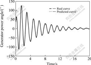
Fig.1 Comparison of real power angle curve with predicted power angle curve in stable condition

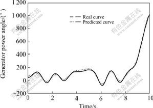
Fig.2 Comparison of real power angle curve with predicted power angle curve in unstable condition

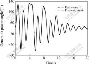
Fig.3 Comparison of real power angle curve with predicted power angle curve in regulated condition

Table 1 Comparison of proposed method and traditional LS-SVM in different time windows

6 Conclusions

1) The recursive algorithm for inverting block matrix is used to modify the traditional LS-SVM.

2) Based on this method, the storage space and the training time of support vectors are reduced remarkably. The computing speed of the proposed method is nearly not affected by the size of sample set.

3) Compared with the traditional LS-SVM in same time window, the proposed method has the same generalization ability and prediction accuracy.

4) By applying the proposed method to power system transient stability prediction, the results indicate that the algorithm is characterized by stronger learning ability than standard LS-SVM and suitable for time series online prediction.

References

[1] KUGIUMTZIS D, LINGIARDE O C, CHRISTOPH-ERSEN N. Regularized local linear prediction of chaotic time series[J]. Physica D, 1998, 11(2): 344-360.

[2] WHITEHEAD B A, CHOATE T D. Cooperative-competitive genetic evolution of radial basis function centers and widths for time series prediction[J]. IEEE Transactions on Neural Networks, 1996, 7(4): 869-880.

[3] YEE P, HAYKIN S. A dynamic regularized radial basis function network for nonlinear, nonstationary time series prediction[J]. IEEE Transactions on Signal Processing, 1999, 47(9): 2503-2521.

[4] GENCAY R, LIU T. Nonlinear modeling and prediction with feedforward and recurrent networks[J]. Physica D, 1997, 10(8): 119-134.

[5] YU Li-xin, ZHANG Yan-qing. Evolutionary fuzzy neural networks for hybrid financial prediction[J]. IEEE Transactions on Systems, Man and Cybernetics, Part C, 2005, 35(2): 244-249.

[6] GHAZALI R, HUSSAIN A, EL-DEREDY W. Application of ridge polynomial neural networks to financial time series prediction[C]// International Joint Conference on Neural Networks. Vancouver, BC, Canada : Tyndale House Press, 2006: 235-239.

[7] VAPNIK V N. The Nature of Statistical Learning Theory[M]. New York: Spring-Verlag Press, 1995.

[8] CHERKASSKY V, MULIER F. Learning from Data-Concepts: Theory and Methods[M]. New York: John Wiley Sons Press, 1998.

[9] JOACHIMS T. Text categorization with support vector machines: learning with many relevant features[C]// Proceedings of the European Conference on Machine Learning(ECML). Paris: John Wiley Sons Publisher, 1998: 137-142.

[10] GUYON I, WESTON J, BARNHILL S. Gene selection for cancer classification using support vector machines[J]. Machine Learning, 2002, 46(1): 389-422.

[11] HE Xue-wen, ZHAO Hai-ming. Support vector machine and its application to machinery fault diagnosis[J]. Journal of Central South University of Technology: Natural Science, 2005, 36(1): 97-101. (in Chinese)

[12] ZHONG Wei-min, PI Dao-ying, SUN You-xian. Support vector machine based nonlinear model multi-step-ahead optimizing predictive control[J]. Journal of Central South University of Technology, 2005, 12(5): 591-595.

[13] KIVINEN J, SMOLA A, WILLIAMSON R. Online learning with kernels: Advances in Neural Information Processing Systems[M]. Cambridge, MA: MIT Press, 2002.

[14] RALAIVOLA L. Incremental support vector machine learning: A local approach[C]// Proceedings of the International on Conference on Artificial Neural Networks. Vienna: St Martin Publisher, 2001: 322-329.

[15] KUH A. Adaptive kernel methods for CDMA systems[C]// Proceedings of the International Joint Conference on Neural networks. Washington DC: Spring-Verlag Publisher, 2001: 1404-1409.

[16] SUYKENS J, VANDEWALE J. Least squares support vector machine classifiers[J]. Neural Processing Letters, 1999, 9(3): 293-300.

(Edited by CHEN Wei-ping)

                     

Foundation item: Project (SGKJ[200301-16]) supported by the State Grid Cooperation of China

Received date: 2006-10-18; Accepted date: 2006-12-18

Corresponding author: WU Qiong, Doctoral candidate; Tel: +86-10-51971466; E-mail: bjwq7972@126.com