J. Cent. South Univ. (2016) 23: 449-460

DOI: 10.1007/s11771-016-3090-4

hybrid reliability model for fatigue reliability analysis of steel bridges

CAO Shan-shan(曹珊珊), LEI Jun-qing(雷俊卿)

School of Civil Engineering, Beijing Jiaotong University, Beijing 100044, China

Central South University Press and Springer-Verlag Berlin Heidelberg 2016

Abstract: A kind of hybrid reliability model is presented to solve the fatigue reliability problems of steel bridges. The cumulative damage model is one kind of the models used in fatigue reliability analysis. The parameter characteristics of the model can be described as probabilistic and interval. The two-stage hybrid reliability model is given with a theoretical foundation and a solving algorithm to solve the hybrid reliability problems. The theoretical foundation is established by the consistency relationships of interval reliability model and probability reliability model with normally distributed variables in theory. The solving process is combined with the definition of interval reliability index and the probabilistic algorithm. With the consideration of the parameter characteristics of the S-N curve, the cumulative damage model with hybrid variables is given based on the standards from different countries. Lastly, a case of steel structure in the Neville Island Bridge is analyzed to verify the applicability of the hybrid reliability model in fatigue reliability analysis based on the AASHTO.

Key words: hybrid reliability model (HRM); consistency relationships; linear and bilinear S-N curve; fatigue reliability; normal distribution

1 Introduction

Fatigue failure is a common form of structural destruction in the field of civil engineering. The fatigue reliability analysis of the structure can be influenced from the physical dimensions, the machining precisions, the loadings and the environmental conditions. However, the requirements of the endurance tests are quite high, especially in the facility, the specimen processing level, and the cost of capital. The numbers of the effective samples in fatigue tests cannot satisfy the needs of the statistics. The conventional probability reliability analysis with the parameters that lack of sample data can produce immeasurable errors [1-2], which cannot meet the precision in engineering.

BEN-HAIM and ELISHAKOFF [1-2] proposed the concept of the non-probabilistic approach to obtain the reliability of structures. ELISHAKOFF et al [3-4] deemed that the non-probabilistic reliability belonged to an interval and the reliability index, which was also an interval quantity based on the interval theory. GUO et al [5] proposed a non-probabilistic measure and methodology for the structural reliability computation, and considered the physical significance of evaluation index of the nonprobability reliability index η the minimum distance from the origin to the failure plane.

In order to make full use of existing statistical data, the scholars put forward the hybrid reliability model (HRM) with interval variables and the probability variables [6-8]. And two kinds of algorithms were developed for the solution of the HRM. GUO and LU [6] first proposed a hybrid reliability analysis method with a two-stage performance function to solve the linear problems, which considered both the interval reliability model (IRM) and the probabilistic reliability model (PRM). This method needs high consistency between two type models. QIAO [9] ever proved the compatibility between the convex set model and the PRM with uniformly distributed variables, and discussed the relationship between the IRM and the convex set model. WANG and QIU [10] ever proved the compatibility between the stress strength interference non-probability model and the PRM with uniformly distributed variables. However, the common forms of distributions of the uncertainty such as normal were not considered, and the relationship between the IRM and the PRM was not explored with some universal direct expressions.

Besides, in the development of solving process in the HRM, LI et al [11] converted uncertain parameters of the hybrid model to the non-probability, and defined the reliability index with the non-probabilistic reliability method. PENMETSA and GRANDHI [12] and GUO and LU [6] used the failure probability to describe the HRM without discussing the reliability index. LUO et al [13] explored the relationship between the reliability indices of the PRM and the HRM with the convex set model without the specific explanation of the influence of interval variables on its evaluation criterion. Jiang et al discussed the computational efficiency and precision between the PRM and the HRM based on the optimization theory, and analyzed the correlation among the variables [14]. It was observed that there is no reference in the consistency between the IRM and the PRM with normally distributed variables in the existing study on the hybrid model. And there is no reasonable theoretical explanation of the evaluation index of the HRM; while, the normal distribution is the essential distribution form, and the reliability index is the most commonly evaluation index in the engineering. The lack of the two parts limits the application of the hybrid reliability in civil engineering.

The main objective of this work is to provide a two-phase hybrid reliability model to assess and predict the fatigue life of steel structures based on the linear cumulative damage model. Firstly, the theoretical foundation and a solving algorithm of the two-phase hybrid reliability model are given in this work to solve the hybrid reliability problems with probabilistic variables and interval variables. Secondly, the parameters of the model that contains linear or bilinear S-N curve are distinguished as probabilistic variables and interval variables. Finally, a case of fatigue category C in the Neville Island Bridge is analyzed to discuss the applicability of the hybrid reliability model in fatigue evaluation based on the AASHTO.

2 theoretical foundation in reliability model

The HRM is built on the consistency relationship of the PRM and the IRM that is acquired by theoretical derivation and verified by a ternary linear numerical case.

2.1 Definition and assumptions

The PRM contains only random variables [15], and the IRM, one kind of non-probability model, contains only interval variables. There are four assumptions as follows to simplify the calculation in this theoretical derivation.

1) All the variables are assumed independent with each other.

2) The first-order second-moment method is adopted to deal with the PRM.

3) The defining method is adopted to deal with the IRM.

4) There are n variables in the structural reliability model, which contains the resistance R and the load effects S_i (i=1, 2, …, n-1).

2.2 Consistency of PRM and IRM

Considering the above assumptions, the performance function is defined as Eq. (1). If all the variables in the function are normally distributed, the reliability index of PRM (PRI) can be estimated as Eq. (2).

(i=1, 2, …, n-1)            (1)

                        (2)

where μ_R and s_R are the mean and standard deviations of the resistance R and R~N(μ_R, );  and  are the mean and standard deviation of the load effects S_i and S_i~N();  is the safety factor; γ_R=s_R/μ_R and  are the variation coefficients (COV) of the resistance R and the load effects S_i.

If all the variables in the function are transformed into the interval variables, and the ranges of interval are and   m_R and  (i=1, 2, …, n-1) are the deviation coefficients of variables, and m_R>0, >0. μ_R and  (i=1, 2, …, n-1) are the means of the interval variables, and Δ_R=m_Rs_R  and  (i=1, 2, …, n-1) are the dispersions of the interval variables. Based on the concept of safety factor in the PRM, the safety factor of interval analysis can be expressed as Eq. (3). The variation coefficients can be expressed as Eq. (4).

     (3)

         (4)

Combining with the definition of interval reliability [5], the interval reliability index (IRI) can be acquired as

         (5a)

where  () is the coefficient of load participation. Based on Eq. (5a), η could be distinctly expressed by the PRI β and some parameters used in the PRM (K_m, γ_R,  Especially, when  the IRI is rewritten as

              (5b)

It can be seen that the relationship between the IRI and the PRI relies on m and a ratio that is less than 1.0, which can be described as η<β/m.

The deviation coefficients of variables are commonly assumed to be equal,  And the different kinds of random variable distributions can be transformed into the normal distribution. Then it can be concluded that the restricted condition of the equation η<β/m is necessary in solving the interval reliability model.

2.3 Validation example

A ternary linear function of structure [16] is proposed as

                               (6)

The characteristics of the resistance R and the effects S₁ and S₂ are listed in Table 1.

Table 1 Details of parameters and results of reliability model of Eq. (6)

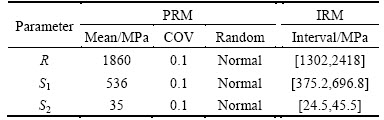
For the PRM, the reliability index is obtained by Eq. (2) and β=6.657. Then, the IRI is obtained according to Eq. (5) in theory. The expression is rewritten as

      (7)

where the safety factor is K_m=3.257 and the coefficient of load participation is  The positive coefficients of the dispersion  are assumed to be constrained by two boundaries (from 1 to 3), whose determinations are based on 3-standard deviation (3s) criterion. The variation tendency of the IRI can be presented as Fig. 1. It can be observed that the IRI is decreased with the increase of  But the amplitudes of the variations are quite different. It can be confirmed that this difference on the IRI depends on the coefficients of load participation α_i. In this case, the positive coefficients of the dispersion are uniformly assumed as 3.0, where the influence on evaluation is relatively small.

The IRI of this case can be acquired by three methods, the modified one-dimensional optimization algorithm (ODOA) [17], the multi-dimensional optimization algorithm and affine projection algorithm (APA) [18], and the formula calculation of Eq. (5). The results by the three methods are 1.767, 1.767 and 1.776, respectively. The calculation error among these three methods is 0.507%<5%, which meets the accuracy requirement. The relational expression proposed in Eq. (5) is tenable.

3 Hybrid reliability model (HRM) and solution algorithms

3.1 basic definition model

The HRM contains both of the random variables (X={X₁, X₂, …, X_n}) and the interval variables (Z={Z₁, Z₂, …, Z_m}), which are assumed to be independent in the study, and the performance function is g_H=g_H(X, Z).

Based on the concept of the HRM with a two-stage performance function [6], the first stage performance function can be expressed as Eq. (8) with the consideration of the interval variables z. Then the reliability index that is associated with the random variables can be obtained by interval algorithm as Eq. (9).

                              (8)

                 (9)

where g_H(X, Z)^c and g_H(X, Z)^r are the mean and deviation of g_H(X, Z), respectively.

Then, the second stage performance function is established as Eq. (10), and the structure is safe if  The final reliability index of the HRM (HRI) is represented as Eq. (11), where the performance function is transformed from the original space X to the standard normal space Y with a probability transformation function T.

                             (10)

                 (11)

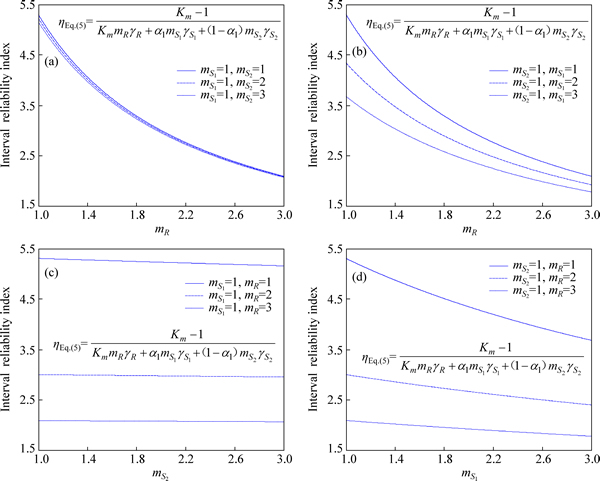
Fig. 1 variation tendency of interval reliability indices with different dispersions

3.2 Simplified model in theory

In particular, a performance function is defined as

         (12)

where R_P and S_P are the normally distributed random variables of the resistance and the effect, which are assumed to be independent, and R_P~N S_P~N  and  are the mean and the standard deviation of R_P.  and  are the mean and the standard deviation of S_P;   are the interval variables;  and  are the mean and the dispersion of R_I;  and  are the mean and the dispersion of S_I. Then, the IRM is firstly analyzed as   Eq. (13). The index η_I is concerned with the random variables R_P and S_P:

               (13)

Then the second stage performance function is established as

     (14)

Based on the JC method, the reliability index of the probability reliability model can be estimated as Eq. (15a). It is also the final hybrid reliability index.

      (15a)

Particularly, if the interval variables are assumed as constant, the PRI of the model is  And if the random variables are assumed as constant, the IRI of the model is  Then, Eq. (15a) can be rewritten as Eq. (15b), which can describe the relationship that the HRM integrates the PRM and the IRM very well.

                (15b)

β_H of the HRM is a more reasonable index to evaluate and predict the safety of structure, which can better reflect both the uncertainty of interval variables and the probability of random variables.

3.3 Solution algorithms

Based on the above theoretical foundation, the establishment and the solving steps of hybrid reliability model are proposed systematically as follows.

Step 1): The establishment of the first stage function,  If  the structure is safe.

Step 2): The classification of the variables in the function. As to the random variables, the distribution form and relevant parameters with enough accuracy should be accessible. As to the interval one, the mean and the dispersion should be available. In the field of civil engineering, most parameters may be assumed to be approximately distributed. If the distribution forms of the assumption are non-uniform, the parameters can be assumed as interval variables with the dispersion acquired by 3s criterion, and the coefficient of dispersion is in the scope of [1, 3]. With the consideration of Eq. (5b), it is necessary to select the right coefficient of dispersion to meet the restriction η<β/m.

Step 3): The solution of the interval reliability model with the random variables is assumed as constant. The interval reliability model in Eq. (16) can be solved by definition method [6], multi-dimensional optimization algorithm (MDOA), the modified one dimensional optimization algorithm (ODOA) [17], affine projection algorithm (APA) [18] and so on.

Step 4): The effectiveness verification of the solution is calculated from Step (3). If  the calculation can be continued to Step 5). If  the Step (3) should be repeated. η_I is the IRI of the model ignoring the random variables, and  is a some value of the random variable X.

Step 5): The establishment of the second stage function with the probability reliability model,  As to the engineering structures, if  the structure is safe.

Step 6): The solution of the probability reliability model. It can be solved by first-order second-moment method (or JC method), Monte Carlo method, response surface method and so on. The probability reliability index β_H is also the finally index of the HRM.

It can be concluded that the restrictions in step (4) is based on the consistency of the PRM and the IRM, which can avoid the interval extension in results caused by the interval operation in nonlinear functions and ensure the effectiveness of solving. The total flowchart is shown in Fig. 2.

4 Fatigue analysis of cumulative damage model

The cumulative damage model based on Miner criterion can be used to express the fatigue limit state before the crack initiation of structure:

                              (16)

where △ is the critical cumulative damage value; D is the actual cumulative damage value; e is the correction coefficient for measurement error.

4.1 S-N Curve

The fatigue reliability assessment of structure is based on the different category S-N curves that can be expressed as Eq. (17) [19] and in Fig. 3.

                                  (17)

where m is the materials parameters on the slope of the curves; A is the parameters of material details; S is the stress amplitude; N is the number of stress cycles.

When the structure is under the variable amplitude loadings, the linear cumulative damage model in Eq. (16) can be translated as Eq.(18).

                     (18)

where n_i is the number of cycles with the stress amplitude S_i; S_eq is the equivalent constant stress amplitude that can be obtained by

                          (19)

As to the fatigue life with low stress amplitude loadings that S_eq≤[S], CONNOR et al [20] analyzed the details with the fatigue test data in the real bridge based on the bilinear S-N curve. CRUDELE and YEN [21] proposed a quadratic linear segment with the slope of 4 in the bilinear S-N curve based on the AASHTO [22]. Kwon et al [23] and SOLIMAN et al [24] discussed the fatigue life of different categories based on the bilinear

S-N curves. YEN et al [26] provided information regarding the development of the new equivalent constant amplitude stress ranges for the bilinear S-N curves. Besides, a multi-segmented S-N curve is given in the Eurocode3 [25]. A uniform of the bilinear S-N curves is proposed as

                       (20)

where [S] is a kind of the constant amplitude fatigue threshold (CAFT) based on the AASHTO or the constant amplitude fatigue limit at 5 million cycles in the Eurocode3; m₁ and m₂ are the slopes of the bilinear S-N curve with the stress amplitude S greater and smaller than [S], respectively.

Fig. 2 calculation flowchart of hybrid reliability model

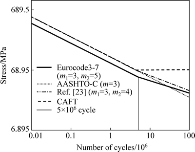
Fig. 3 S-N curve

Based on the Miner criterion, the cumulative damage model with the equivalent constant amplitude S_eqB≤[S] can be translated as

                      (21)

where the equivalent constant amplitude S_eqB can be obtained by

                    (22)

where n_i is the number of cycles with the stress amplitude S_i greater than [S]; n_j is the number of cycles with the stress amplitude S_j smaller than [S];  is the total number of cycles.

4.2 characteristics of parameters

There are several variables (△, e, A, A₁, A₂, S_eq, S_eqB) in the linear damage accumulation model based on the S-N curve. There are some reasonable conclusions in the characteristics about the Δ and the e. As to the metal material, WIRSCHING [27] concluded that the critical cumulative damage value Δ can be described by the logarithmic normal distribution with the mean of 1.0 and variable coefficient of 0.3. FRANGOPOL et al [28] considered that the correction coefficient of measurement errors can be described by the logarithmic normal distribution with the mean of 1.0 and variable coefficient of 0.04 [28].

As to the parameters of material details A(A₁, A₂), there are different values based on different criterions on the S-N curve. In the AASHTO, A₁=A and A₂= and A is the parameters of material details that can be obtained by different category S-N curves. Fisher concluded that A can be assumed as logarithmic normal distribution with fatigue test data of 374 beams. In the AASHTO, the design value of A, A_D has 95% survival probability. According to the statistical theory, A_D, can be acquired with.

                    (23)

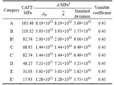
where  s_A and d_A are the mean, the standard deviation and the variable coefficient of A, respectively. WIRSCHING et al [29] proposed that the variable coefficient can be assumed as 0.45. The mean and the standard deviation of various categories in AASHTO are shown in Table 2. In the Eurocode3, the material parameters A₁=C₁=2×10⁶ A₂=C₂=5×10⁶. Δs_C is the detail category at 2×10⁶ cycle. Δs_D is the constant amplitude fatigue limit at 5×10⁶ cycle. And the C₁ and C₂ can be assumed as logarithmic normal distribution.

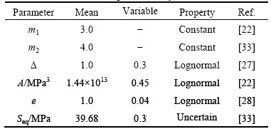
Table 2 values of parameters in AASHTO

As to the characteristics of the equivalent stress amplitudes (S_eq, S_eqB), it is feasible to take regression analysis of stress histogram based on the monitoring data [30]. ZHAO et al [31] used Rayleigh distribution to describe the characteristics of the equivalent stress amplitude. XIA et al [32] pointed out that stress histogram cannot be described by a single distribution model based on the monitoring data of Tsing Ma Bridge. KWON and FRANGOPOL [33] considered S_eq the random variable, and analyzed the difference between the fatigue reliability indices when S_eq was assumed as different distributions. What’s more, the valid data are inaccessible for the bridges constructed early with lack of monitoring system. And the distribution characteristic of S_eq is uncertain. The discussions have been taken to analyze the rationality and feasibility when S_eq and S_eqB are assumed as interval variables with examples in real bridge.

5 Application examples

With the consideration of linear and bilinear S-N curve and the two-phase hybrid reliability model in the above analysis, the fatigue life of category C (AASHTO) in the CH-16 of Neville Island Bridge is analyzed to discuss the applicability of the hybrid reliability model in the fatigue reliability analysis. The details of the category C are shown in Fig. 4 [23].

5.1 Linear S-N curve in AASHTO

As to the Neville Island bridge, the average daily truck traffic (ADTT) is 1290 [24]. With the consideration of the annual traffic increase rate of α=2%, the annual traffic is  And the stress amplitude spectrum in Fig. 5 was provided by KWON et al [23]. Combining the Miner’s criterion with the linear S-N curve in AASHTO, the performance function can be presented as Eq. (24) based on Eq. (16) and Eq. (18). The details of the parameters in Eq. (24) are shown in Table 3.

          (24)

The fatigue life of category C (AASHTO) in the CH-16 of Neville Island Bridge is analyzed firstly by the first-order second-moment method. The mean of the equivalent constant stress amplitude S_eq is acquired with 39.68 MPa based on Eq. (19) and Fig. 5. The variable coefficient is assumed as 0.3, and the fatigue reliability evaluation is performed when S_eq is assumed to be lognormal, Weibull, or normal [33]. The results are shown in Fig. 6(a). Compared with the calculations of Ref. [34], where the mean of S_eq is 0.5CAFT and the variable coefficient is 0.3, it is concluded that the fatigue reliability indices are reasonable. Besides, the difference of the fatigue reliability indices is non- ignorable with S_eq in different distributional hypothesis. Especially, the diversity is quite prominent under the former 25×10⁶ cycle. With the consideration of the diversity in variable coefficient, the variation of the fatigue reliability indices can be observed in Fig. 6(b). It can be concluded that the reliability indices of the same cycles will be smaller if the variable coefficient is higher. And the diversity is alsoquite prominent under the former 25×10⁶ cycle.

Fig. 4 details of category C

Fig. 5 Frequency of stress range

Table 3 parameters for fatigue reliability model

Then, the fatigue life of category C is also be analyzed by the HRM in Fig. 2. The parameter S_eq is taken as the interval variable with the dispersion coefficient of 1.0. The basic interval is [27.776, 51.584]. The other variables are adopted the same in Table 3. The hybrid reliability indices are calculated in Fig. 6(c) of HRI curve. It can be observed that the descending slop of the HRI is much higher than the one of the PRI with the increase of cycles. With the consideration of the diversity in variable coefficient or interval range, the variation of the HRI of fatigue life can be observed by Fig. 6(d). It can be concluded that the reliability index of the same cycles will be smaller if the variable coefficient or interval range is larger. And the diversity is quite prominent after the 25×10⁶ cycle, which may be more reasonable to explain the phenomenon that the fatigue damage cumulative effect of structure is more aggravated with the increase of loading cycles. The rule of the hybrid reliability index is closer to the practical situation.

Fig. 6 Reliability indices of models with linear S-N curve:

5.2 Bilinear S-N curve

As ,the performance function can be represented as Eq.(25) based on Miner’s criterion with the bilinear S-N curve and Eq.(16) and Eq.(21).

where the characteristics of △, e, N and m₁ are shown in Table 3, and m₂=4 [21]. The mean value of the equivalent constant stress amplitude S_eqB is acquired with 42.12 MPa based on Eq.(22). The variable coefficient of S_eqB is assumed as 0.3, and the fatigue reliability evaluation is performed when S_eqB is assumed to be lognormal, Weibull, or normal [33]. The results are shown in Fig. 7(a). The difference of the fatigue reliability indices is non-ignorable with S_eqB in different distributional hypothesis. Especially, the diversity is quite prominent under the former 25×10⁶ cycle. With the consideration of the diversity in variable coefficients, the variation of the fatigue reliability indices can be observed in Fig. 7(b). It can be concluded that the reliability indices of the same cycles are smaller when the variable coefficient is larger. And the diversity is decreased with the increase of loading cycles.

Then, the fatigue life of category C is also be analyzed by the HRM in Fig. 2. The parameter S_eqB is taken as the interval variable with the dispersion coefficient of 1.0. The basic interval is [29.484, 54.756]. The other variables are adopted the same in Table 3. The hybrid reliability indices are calculated in Fig. 7(c) of the HRI curve. It can be observed that the descending slop of the HRI is much higher than the one of the PRI with the increase of cycles. With the consideration of the diversity in dispersion or interval range, the variation of the HRI of fatigue life can be observed in Fig. 7(d). It can be concluded that the reliability indices of the same cycles are smaller if the variable coefficient or interval range is larger. And the diversity is increased with the increase of loading cycles, which may be more reasonable to explain the phenomenon that the fatigue damage cumulative effect of structure is more aggravated with the increase of loading cycles. The rule of the hybrid reliability indices is closer to the practical situation.

5 Discussions

Based on survival probability of 95%, a target reliability index of 1.65 is assumed implying a failure probability of approximately 0.05. If fatigue life of structures is predicted based on the target reliability index of 1.65, the comparisons of the HRI and the PRI are shown in the Fig. 8. It can be observed some conclusions. As to the reliability indices of the models with linear S-N curve in Fig. 8(a), when the variable coefficients of S_eq in two models are 0.3 and 0.35, the fatigue life predicted by the HRM is shorter than the one predicted by the PRM; While, when the variable coefficients are 0.4, 0.45 and 0.5, the fatigue life predicted by the HRM is longer than the one predicted by the PRM. It concluded that the fatigue life prediction by the HRM is much more conservative when the variable coefficient of S_eq is smaller than 0.35.

Fig. 7 Reliability indices of models with bilinear S-N curve:

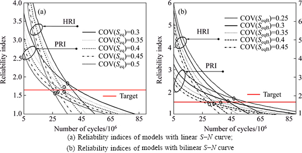
Fig. 8 comparison diagram of reliability indices:

As to the reliability indices of the models with bilinear S-N curve in Fig. 8(b), when the variable coefficients of S_eqB in the PRM and in the HRM are 0.25, 0.3 and 0.35, the fatigue life predicted by the HRM is shorter than the one predicted by the PRM; While, when the variable coefficients of S_eqB in two models are 0.4 and 0.45, the fatigue life predicted by the HRM is longer than the one predicted by the PRM. It concluded that if the variable coefficient S_eqB is smaller than 0.35, the fatigue life prediction by the HRM is much more conservative.

6 Conclusions

1) A hybrid reliability model is presented to solve the fatigue reliability problems of steel structures. The theoretical foundation of the HRM is established by the consistency relationships of interval reliability model and probability reliability model with normally distributed variables in theory. The solving process combined with the definition of interval reliability index and the probabilistic algorithm is efficient and reliable.

2) In the linear damage accumulation model that contains linear S-N curve or bilinear S-N curve, the variability and the uncertainty of S_eq and S_eqB cannot be ignored.

3) The two-phase hybrid reliability model can be used in the fatigue life prediction with a scope of application. Based on the application example, the analysis results of fatigue reliability with the HRM may be more reasonable to explain the phenomenon that the fatigue damage cumulative effect of structure is more aggravate with the increase of loading cycles. And when the variable coefficient of S_eq in the linear S-N curves and the variable coefficient of S_eqB in the bilinear S-N curves are smaller than 0.35, the fatigue life prediction by the HRM is much more conservative than the one predicted by the PRM.

References

[1] BEN-HAIM Y, ELISHAKOFF I. Convex models of uncertainties in applied mechanics [M]. Amsterdam: Elsevier Science, 1990.

[2] BEN-HAIM Y. A non-probabilistic concept of reliability [J]. Structural Safety, 1994, 14(4): 227-245.

[3] ELISHAKOFF I, COLOMBI P. Combination of probabilistic and convex models of uncertainty when limited knowledge is present on acoustic excitation parameters [J]. Comput Methods Appl Mech Eng, 1993, 104: 187-209.

[4] ELISHAKOFF I, CAI G Q, STAMES J H. Non-linear buckling of a column with initial imperfections via stochastic and non-stochastic convex models [J]. Int J Nonlin Mech, 1994, 29: 71-82.

[5] GUO Shu-xiang, LU Zhen-zhou, FENG Yuan-sheng. A non-probabilistic model of structure reliability based on interval analysis [J]. Journal of Computational Mechanics, 2001, 18(1): 56-60. (in Chinese)

[6] GUO Shu-xiang, LU Zhen-zhou. Hybrid probabilistic and non-probabilistic model of structural reliability [J]. Chinese Journal of Mechanical Strength, 2002, 24(4): 524-526, 530. (in Chinese)

[7] GUO Jia, DU Xiao-ping. Reliability sensitivity analysis with random and interval variables [J]. International Journal for Numerical Methods in Engineering, 2009, 78: 1585-1617.

[8] JIANG C, LI W X, HAN X, LIU L X, LE P H. Structural reliability analysis based on random distributions with interval parameters [J]. Computers and Structures, 2011, 89: 2292-2302.

[9] QIAO Xin-zhou. Uncertain structural reliability analysis and optimization design research [D]. Xi’an: Xi’an Electronic and Engineering University, 2008. (in Chinese)

[10] WANG Jun, QIU Zhi-ping. Probabilistic and non-probabilistic hybrid reliability model of structures [J]. Aeronautica et Astronautica Sinica, 2009, 30(8): 1398-1404. (in Chinese)

[11] LI Kun-feng, YANG Zi-chun, SUN Wen-cai. New hybrid convex model and probability reliability method for structures [J]. Journal of mechanical engineering in Chinese, 2012, 48(14): 192-198. (in Chinese)

[12] PENMETSA R, GRANDHI R. Efficient estimation of structural reliability for problems with uncertain intervals [J]. Computers and Structures, 2002, 80: 1103-1112.

[13] LUO Yang-jun, KANG Zhan, LI Alex. Structural reliability assessment based on probability and convex set mixed model [J]. Computers and Structures 2009, 87: 1408-1415.

[14] JIANG Chao, ZHENG Jing, HAN Xu, ZHANG Qing-fei. A probability and interval hybrid structural reliability analysis method considering parameters’ correlation [J]. Chinese Journal of Theoretical and Applied Mechanics, 2014, 46(4): 591-600. (in Chinese)

[15] LIU Yong-jun, FAN Jin-wei, LI Yun. Reliability evaluation method and algorithm for electromechanical product [J]. Journal of Central South University, 2014, 21(10): 3753-3761.

[16] CAO Shan-shan, LEI Jun-qing, ZHANG Kun. The non-probabilistic reliability analysis of stayed-cable based on the interval algorithm [J]. Applied Mechanics and Materials, 2014, 455: 267-273.

[17] CHEN Xu-yong. Reliability investigation of RC bridge in-service based on non-probabilistic theoretical model [D]. Wuhan: Huazhong University of Science and Technology, 2010. (in Chinese)

[18] JIANG Tao, CHEN Jian-jun, ZHANG Chi-jiang. Non-probabilistic reliability index and affine arithmetic [J]. Journal of Mechanical Strength, 2007, 29(2): 251-255. (in Chinese)

[19] FISHER J W. Fatigue and fracture in steel bridges [M]. New York: John Willey and Sons, 1984.

[20] CONNOR R J, HODGSON I C, MAHMOUD H N, Bowman C A. Field testing and fatigue evaluation of the I-79 Neville Island bridge over the Ohio River [R]. Bethlehem, PA: Lehigh Universiey, Center for Advanced Technology for Large Structural Systems (ATLSS), 2005.

[21] CRUDELE B B, YEN B T. Analytical examination of S-N curves below constant amplitude fatigue limit [C]// Proc 1st Int Conf on Fatigue and Fracture in the Infrastructure. Bethlehem, PA: ATLSS Engineering Research Center, Lehigh University, 2006.

[22] AASHTO Guidelines, AASHTO Standard Specification [S]. 6th ed for highway bridges. Washington: American Association of State Highway and Transportation Officials, 2012.

[23] KWON K, FRANGOPOL D M, SOLIMAN M. Probabilistic fatigue life estimation of steel bridges by using a bilinear approach [J]. Journal of Bridge Engineering, 2012, 17(1): 58-70.

[24] SOLIMAN M, FRANGOPOL D M, KWON K. Fatigue assessment and service life prediction of existing steel bridges by integrating SHM into a probabilistic bilinear S-N approach [J]. J Struct Eng, 2013, 139: 1728-1740.

[25] BSI. BS EN 1993-1-9 -2005 Eurocode 3: Design of steel structures Part 1. 9: Fatigue [S]. London: British Standards Institution, 2006.

[26] YEN B T, HODGSON I C, EDWARD Z Y, CRUDELE B B. Bilinear S-N curves and equivalent stress ranges for fatigue life estimation [J]. Journal of Bridge Engineering, 2013, 18(1): 26-30.

[27] WIRSCHING P H. Fatigue reliability for offshore structures [J]. Journal of Structural Engineering, ASCE, 1984, 110(10): 2340-2356.

[28] FRANGOPOL D M, STRAUSS A, KIM S. Bridge reliability assessment based on monitoring [J]. Journal of Bridge Engineering, ASCE, 2008, 13(3): 258-270.

[29] WIRSCHING P H, ORTIZ K, CHEN Y N. Fracture mechanics fatigue model in a reliability format [C]// Proc 6th Int Syrup on OMAE. Houston, TX: OMAE, 1987.

[30] LIU M, FRANGOPOL D, KWON K. Fatigue reliability assessment of retrofitted steel bridges integrating monitored data [J]. Structural Safety, 2010, 32(1): 77-89.

[31] ZHAO Z W, HALDAR A, BREEN F L. Fatigue-reliability evaluation of steel bridges [J]. Journal of Structural Engineering, ASCE, 1994, 120(5): 1608-1623.

[32] XIA H, NI Y, WONG K, KO J M. Reliability-based condition assessment of in-service bridges using mixture distribution models [J]. Computers & Structures, 2012, 106(5): 204-213.

[33] KWON, K, FRANGOPOL D M. Bridge fatigue reliability assessment using probability density functions of equivalent stress range based on field monitoring data [J]. International Journal of Fatigue, 2010, 32(8): 1221-1232.

[34] KWON K, FRANGOPOL D M. Bridge fatigue assessment and management using reliability-based crack growth and probability of detection models [J]. Probabilistic Engineering Mechanics, 2011, 26: 471-480.

(Edited by YANG Hua)

Foundation item: Projects(51178042, 51578047) supported by the National Natural Science Foundation of China; Project(C14JB00340) supported by the Innovative Research Fund in Beijing Jiaotong University, China; Project(2014-ZJKJ-03) supported by Science and Technology Research and Development Fund of the China Communications Construction Co., LTD

Received date: 2015-04-13; Accepted date: 2015-07-14

Corresponding author: LEI Jun-qing, Professor, PhD; Tel: +86-10-51683769; E-mail: jqlei@bjtu.edu.cn, oconan@163.com