J. Cent. South Univ. (2017) 24: 127-136

DOI: 10.1007/s11771-017-3415-y

Modeling of rough surfaces with given roughness parameters

ZHOU Wei(周炜)¹, TANG Jin-yuan(唐进元)^{2, 3}, HE Yan-fei(何艳飞)^{2, 3}, ZHU Cai-chao(朱才朝)⁴

1. Intelligent Manufacturing Institute (Hunan Provincial Key Laboratory of High Efficiency and Precision Machining of Difficult-to-Cut Material), Hunan University of Science and Technology, Xiangtan 411201, China;

2. State Key Laboratory of High Performance Complex Manufacturing, Central South University,

Changsha 410083, China;

3. School of Mechanical and Electrical Engineering, Central South University, Changsha 410083, China;

4. State Key Laboratory of Mechanical Transmission, Chongqing University, Chongqing 400044, China

 Central South University Press and Springer-Verlag Berlin Heidelberg 2017

Abstract: Modeling of rough surfaces with given roughness parameters is studied, where surfaces with Gaussian height distribution and exponential auto-correlation function (ACF) are concerned. A large number of micro topography samples are randomly generated first using the rough surface simulation method with FFT. Then roughness parameters of the simulated roughness profiles are calculated according to parameter definition, and the relationship between roughness parameters and statistical distribution parameters is investigated. The effects of high-pass filtering with different cut-off lengths on the relationship are analyzed. Subsequently, computing formulae of roughness parameters based on standard deviation and correlation length are constructed with mathematical regression method. The constructed formulae are tested with measured data of actual topographies, and the influences of auto-correlation variations at different lag lengths on the change of roughness parameter are discussed. The constructed computing formulae provide an approach to active modeling of rough surfaces with given roughness parameters.

Key words: micro topography; rough surface; roughness; active modeling

1 Introduction

Seeking potential design space from the micrometer scale has become a trend for mechanical design. The qualitative relation between surface micro topography and interface performance has been explored by virtue of the experimental method [1, 2]. To establish a quantitative mapping rule between micro topography and interface performance, simulation and modeling of micro topographies is required. Currently, two dimensional roughness profile parameters are widely used in characterization, evaluation and aided design of micro topographies on component surfaces [3, 4]. Especially, parameters such as Arithmetic average height R_a, root mean square roughness R_q, mean spacing at mean line S_m, mean spacing of adjacent local peaks S, root mean square (RMS) slope σ_m and RMS curvature σ_k are much commoner. Therefore, how to realize rough surface modeling with these given parameters is crucial to analysis and design of micro topographies.

Due to the characteristics of randomness and irregularity, modeling of micro topographies is mainly based upon their height distribution and auto-correlation distribution (ACF) parameters from the statistical sense. In order to model a micro topography with given roughness parameters, it is essential to determine the mapping relation between roughness parameters and statistical distribution parameters. However, modeling based on measured sample data [5] is expensive, and the general statistical characteristics of the micro topography cannot be reflected. Thus, this method fails to establish the expected relation. With the computing formulae [6] derived from the random process theory, the relation can be obtained, but the roughness parameters are only those related to central moments of surface power spectral density (PSD), such as RMS slope σ_m and RMS curvature σ_k. The relation between other roughness parameters and statistical distribution parameters is still unknown. Furthermore, it is reported that the random process theory method has principle error [7]. To build the relationship of more roughness parameters to statistical distribution parameters, MANESH et al [8] has derived the relation of the fastest decay autocorrelation length S_al and texture aspect ratio S_tr to correlation length β on the basis of autocorrelation distribution, by which the modeling of the two parameters was achieved. Moreover, for Gaussian surfaces, there exists the relationship R_a=0.8σ between Arithmetic average height R_a and standard deviation σ as well as the relationship R_q=σ between RMS roughness R_q and standard deviation σ [9]. Nevertheless, the mapping relations of parameters like mean spacing at mean line S_m and mean spacing of adjacent local peaks S to statistical distribution parameters are expected to be resolved.

Therefore, this work is devoted to addressing the modeling of rough surfaces based on common roughness parameters by studying their relations to statistical distribution parameters for surfaces with Gaussian height distribution and exponential ACF which are common in engineering. PAWAR et al [10] concluded from their study of micro topography peak distribution that the results directly calculated from the definition of roughness parameters are most stable. Hence, a large number of micro topography samples are randomly generated first using the rough surface simulation method with FFT, and then roughness parameters of the simulated roughness profiles, including mean spacing at mean line S_m, mean spacing of adjacent local peaks S, RMS slope σ_m, RMS curvature σ_k and band width coefficient α, are calculated according to their definition. Therefrom, the relationship between roughness parameters and statistical distribution parameters (standard deviation and correlation length) is investigated. Furthermore, computing formulae of roughness parameters based on standard deviation and correlation length are constructed with the mathematical regression method, and the constructed formulae are tested with experiment data. Finally, a simulation example is provided to showcase the application of the constructed formulae to modeling of rough surfaces with given roughness parameters.

2 Principle and method

Assume that the magnitude and space properties of the micro topography are characterized by height distribution and ACF. For Gaussian surfaces of exponential ACF, the statistical distribution characteristics are determined by standard deviation σ and correlation length β. Therefore, various surfaces show different combinations of σ and β in fact. The rough surface simulation method is first adopted to randomly generate a large number of samples with diverse σ and β. Then the roughness parameters of simulated samples are calculated according to parameter definition. In such a way, the mapping relation of roughness parameters to statistical distribution parameters can be found. The computing formulae of roughness parameters are finally constructed with the mathematical regression method. The main flowchart is shown in Fig. 1.

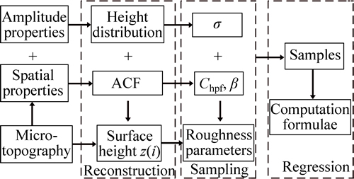
Fig. 1 Main flowchart of method

The FFT rough surface simulation method is adopted in this work, and its relevant principle is referred to Refs. [11, 12]. The expression of exponential ACF is

                       (1)

where R is auto-correlation; τ is lag length; C_hpf is high pass filtering constant; σ and β are standard deviation and correlation length, respectively. WHITEHOUSE and ARCHARD [13] defined correlation length as the distance at which R decayed to 1/10 of the origin value. Thus, C_hpf in Eq. (1) is equal to -2.3. To eliminate the instability caused by long-wavelength components, HIRST and HOLLANDER [14] defined correlation length as the distance when R is equal to 1/e of the value of the origin. Now C_hpf is -0.844. Besides, C_hpf being -1 is used by ARAMAKI et al [15]. Different choices of C_hpf mean doing high-pass filtering with different cut-off lengths. This is discussed in detail in Ref. [9]. The comparison of these three ACFs with different values of C_hpf is shown in Fig. 2. It can be seen that the correlation decays faster when C_hpf is larger. -0.844, -1 and -2.3 are selected for C_hpf to discuss the effect of different values on the calculation results.

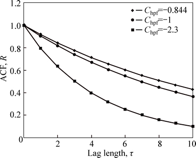
Fig. 2 Comparison of different auto-correlation distributions (β=10)

Surface heights z(i) can be obtained by the convolution of random sequence η(i) with desired height distribution and ACF coefficient matrix a

                         (2)

where a(k) are the coefficients to be determined according to desired ACF, η(i+k) are independent and have unit variance, and n is equal to β+1. Taking the Fourier transform of both sides of Eq. (2) gives

                          (3)

where Z(ω) and A(ω) are Fourier transforms of [z] and [η], respectively. The frequency response H(ω) is H(ω)=. With the determination of H(ω) and A(ω)

from the given statistical distributions, surface heights can then be obtained by the inverse Fourier transform of Eq. (3).

The definitions and computing methods for roughness parameters are provided in Ref. [3], where adjacent peaks with small height differences are treated as one peak. This is different from the three-point definition [6]. The peak definitions will have an impact on the calculating results of spatial parameters. The three-point definition is adopted here since it is optimal in terms of stability in calculating the number of peaks. Besides, quantization accuracy to four decimal places is chosen to avoid digital errors introduced by different quantization width choices. Furthermore, unit sampling interval is used to calculate spatial roughness parameters. Therefore, actual results will be sampling interval times or its reciprocal’s exponential times of the calculated results.

3 Results

The ACF comparison of samples simulated by the FFT simulation method with theory at different correlation lengths is shown in Fig. 3. It is obvious that the simulation program devised in this work has good simulation accuracy. Due to random error, there exist small differences in ACF for a small portion of the samples with the theoretical values. To reduce the impact of random error, 100 samples are randomly simulated for the same σ and β to calculate roughness parameters. The means of the 100 samples are taken as the final results.

The variations of S_m with correlation length under different values of σ and C_hpf are shown in Fig. 4. It is clear that S_m increases gradually with correlation length and finally approaches a constant. S_m has nothing to do with σ. S_m converges faster with a larger C_hpf, and the convergence value decreases with the increase of C_hpf.

The variations of S with correlation length under different values of σ and C_hpf are shown in Fig. 5. The monotonicities of S vary for different values of C_hpf. However, S will finally approach a constant in all cases.S increases with the decrease of correlation length for C_hpf being -0.844 and -1 while it increases with correlation length for C_hpf being -2.3, and the convergence values in the former two cases are smaller than that in the latter case. Moreover, S also has nothing to do with σ.

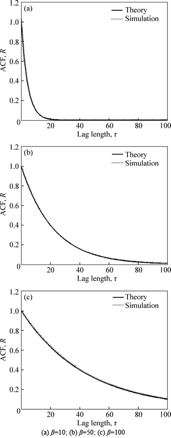
Fig. 3 ACF comparison of simulated samples with theory (C_hpf=-2.3):

The variations of σ_m with correlation length under different values of σ and C_hpf are shown in Fig. 6. σ_m gradually decreases as correlation length increases, and finally reaches a constant; σ_m increases linearly with σ. The larger C_hpf is, the faster σ_m converges and the greater the convergence value will be.

The variations of σ_k with correlation length under different values of σ and C_hpf are shown in Fig. 7. σ_k decreases with the increase of correlation length and finally approaches a constant. It also grows linearly with σ. Like σ_m, σ_k converges faster with a larger C_hpf and a greater convergence value will be obtained for a larger C_hpf.

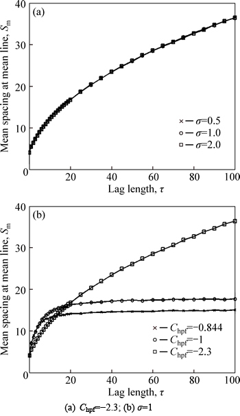
Fig. 4 Variations of S_m with correlation length:

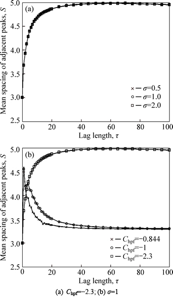
Fig. 5 Variations of S with correlation length:

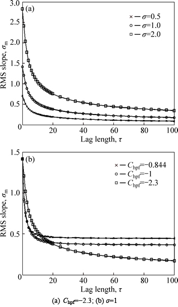
Fig. 6 Variations of σ_m with correlation length:

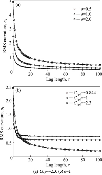
Fig. 7 Variations of σ_k with correlation length:

The variations of α with correlation length under different values of σ and C_hpf are shown in Fig. 8. α grows with different speeds for various values of C_hpf. For C_hpf being -0.844 and -1, α soon assumes a moderate growth. In contrary, α grows linearly with correlation length for C_hpf being -2.3. α has nothing to do with σ, which means the ratio of the second central moment (square of σ_k) to square of the first central moment (square of σ_m) of PSD will be reduced to keep α unchanged when σ increases.

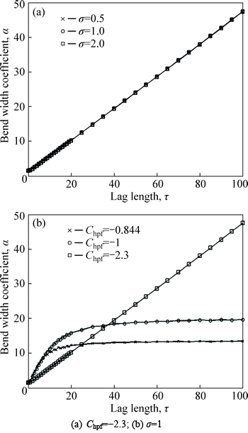
Fig. 8 Variations of α with correlation length:

The computing formulae containing sampling interval △ of the above roughness parameters constructed by the mathematical regression method are as follows

(1) S_m

                        (4)

         (5)

 (6)

(2) S

                         (7)

 (8)

            (9)

(3) σ_m

                        (10)

               (11)

           (12)

(4) σ_k

           (13)

                (14)

           (15)

(5) α

                        (16)

           (17)

        (18)

Jumping occurs at zero for correlation length, which leads the constructed formulae to have relatively large fitting errors here. Take α for example, the simulated result at zero is very close to 1.5, which is consistent with the theoretical value of isotropic Gaussian surface profile obtained from the random process theory method. The calculated result by the constructed formula, however, is only just over 1, which means the relative error is beyond 30%.

4 Experiment validation and discussion

To verify the validity of the aforementioned results, surfaces of four grinding workpieces (Specimen 1-Specimen 4) (shown in Fig. 9(a)) are tested using a Taylor Hobson roughness measuring instrument (shown in Fig. 9(b)). The sampling length is 10 mm, and the sampling interval is 0.5 μm. Four initial tested height sequences are obtained.

In order to facilitate validation, the four initial height sequences are normalized (mean is 0 and standard deviation is 1), and meanwhile the sampling interval is taken as unit size to calculate spatial roughness parameters. The sampling interval is changed for each workpiece to approximatively obtain new tested height sequences of different correlation lengths. The measured profile of Specimen 3 with a sampling length of 10 mm and a sampling interval of 0.5 um is shown in Fig. 10(a), where correlation length is 1298. To obtain tested data with correlation length of 100, the sampling interval iswhere the subscripts of △ indicate correlation length. The new profile is shown in Fig. 10(b). Similarly, a series of tested data with different correlation lengths can be obtained. A part of the profiles are given in Fig. 10.

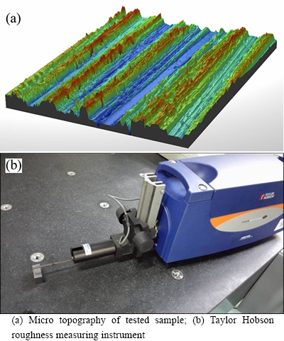
Fig. 9 Topography of tested sample and measuring instrument:

The ACF comparison of tested workpieces with theory under different correlation lengths is shown in Fig. 11.

The variations of roughness parameters with correlation length of the four tested workpieces are compared with those from simulation, as shown in Fig. 12.

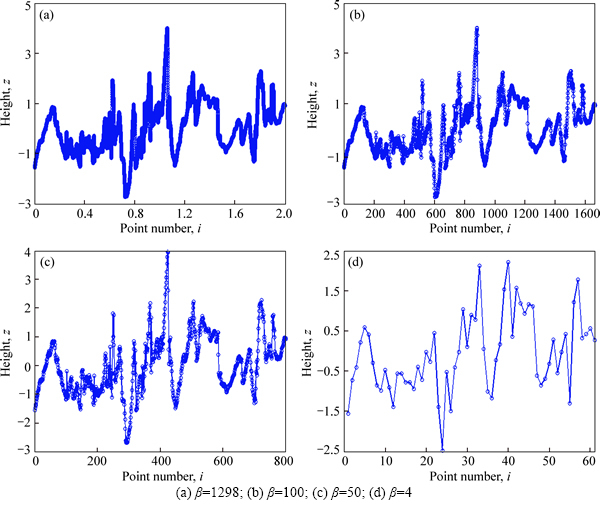
Fig. 10 Profiles of Specimen 3 with different correlation lengths:

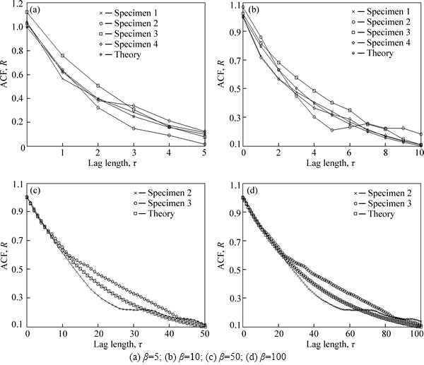
Fig. 11 ACF comparison of tested workpieces with theory (σ=1, C_hpf=-2.3):

It can be seen from Fig. 12 that the simulated values of σ_m, σ_k and α show good consistency with the tested results while there are great differences for S_m and S at large correlation lengths. One reason for the discrepancy is that the workpieces do not obey the ideal exponential ACF and they differ greatly in the intermediate portion of lag lengths as shown in Fig. 11. Another possible reason is that, owing to the interference of the long wavelength components, values of C_hpf for the workpieces are greater than -2.3, which also leads to the deviation.

The differences in ACF between the tested workpieces and theory are dissimilar values of auto- correlation at different lag lengths. To further investigate the causes of the discrepancy between tested results and simulation results, the effect of auto-correlation variations at different lag lengths on roughness parameters is analyzed. As there are multiple roughness parameters, only S_m is discussed as an example. To control the values of R(τ) precisely during the simulation, small correlation lengths (β=5 and β=8) are selected, and the linear transformation algorithm [8], a more accurate method, is used to simulate rough surfaces. Three cases with adjacent differences of △R=0.05 are generated for different lag lengths. Five samples are randomly simulated for the same case to reduce random error. The mean of the five samples is taken as the final result.

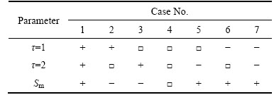
The effects of auto-correlation variations △R on S_m for different lag lengths are shown in Fig. 13. Table 1 and Table 2 list the variations of S_m with △R and with different combinations of △R separately. Thereinto, 7 cases are designed, where Case 1 represents increasing △R both at τ=1 and τ=2 results in the increase of S_m, and so on. It can be found that S_m shows incremental and decremental variation laws with △R when τ=1 and τ=2, respectively. Afterwards, S_m presents a decline trend until it finally fails to give any significant variation rules.

It can still be analyzed from Table 2 that S_m enlarges a little when R continually increases or decreases with τ. This can explain why the values of S_m are both greater than the simulation when Specimen 2 and Specimen 3 show opposite changes relative to the theoretical ACF. Limited by the accuracy of the devised FFT simulation program, auto-correlation R of most of the simulated samples turns out to be continually greater or less than the theory in local areas, though the deviation is small. Thereupon, the calculated results may slightly deviate from the true values.

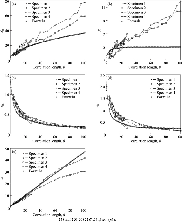
Fig. 12 Comparison of relationship between roughness parameters and correlation length:

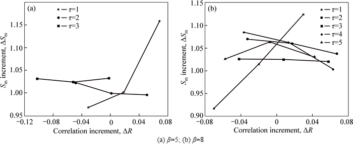
Fig. 13 Effect of auto-correlation variation on S_m for different lag lengths:

Table 1 Variation of S_m with △R (“+”: increase, “-”: decrease, “□”: no rule.)

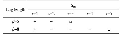
Table 2 Variation of S_m with combinations of △R (β=8), (“+”: increase, “-”: decrease, “□”: R(τ) unchanged)

5 Application

To demonstrate the application of the constructed formulae to rough surface active modeling, RMS slope σ_m and RMS curvature σ_k are taken as the simulation target. Their joint distribution is shown in Fig. 14. The mapping relation of the two parameters with the statistical distribution parameters σ and β is

 (20)

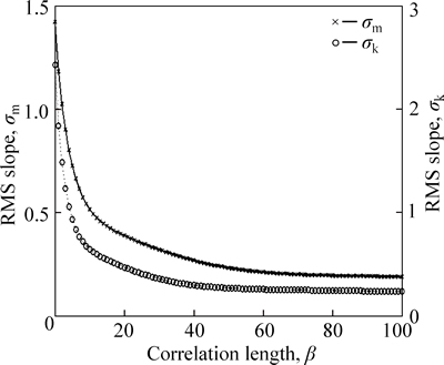
Fig. 14 Joint distribution of RMS slope σ_m and RMS curvature σ_k (σ=1)

Suppose that simulation target is σ_m=0.2 and σ_k=0.2. Taking sampling interval △=1, it can be figured out from Eq. (20) that the ranges of (σ, β) are σ∈(0.6310, 0.7260) and β∈(33, 41). Set σ=0.67 and β=36 will be obtained. Simulate rough surfaces with (σ, β) to model roughness parameters (σ_m, σ_k). Repeat three times randomly. The modeled roughness parameters and the simulation target are compared in Table 3.

Table 3 Comparison of modeled roughness parameters and simulation target

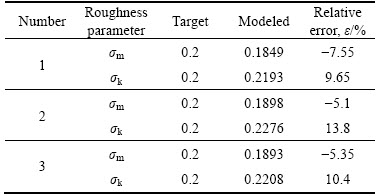
It can be seen from Table 3 that the relative errors of σ_m and σ_k are usually less than 10%. The relative error comes from random error during modeling and the accuracy limitation of the devised simulation program.

6 Conclusions

1) The relation between common roughness parameters and statistical distribution parameters is established. S_m and α increase with correlation length β while σ_m and σ_k decrease with β. The variation of S with β depends upon high pass filtering constant C_hpf. All parameters but band width coefficient α finally converge to constants. σ_m and σ_k increase linearly with standard deviation σ while S_m, S and α have nothing to do with σ. All parameters converge faster with a larger C_hpf, and the convergence values depend upon C_hpf.

2) Computing formulae of roughness parameters are constructed with the mathematical regression method and are tested by experiment. For σ_m, σ_k and α, the simulation results agree well with the tested data, but S_m and S show great differences at large correlation lengths. This is because the surfaces of the tested workpieces do not obey the ideal ACF, and the continuous increase or decrease of auto-correlation leads to the difference between the simulation and the tested results.

3) It is indicated by a simulation example that the constructed formulae can be applied to active modeling of rough surfaces with given roughness parameters.

References

[1] NOVOVIC D, DEWES R C, ASPINWALL D K, VOICE W, BOWEN P. The effect of machined topography and integrity on fatigue life [J]. Int J Mach Tool Manu, 2004, 44(2): 125-134.

[2] FONTE M, ROMEIRO F, FREITAS M. Environment effects and surface roughness on fatigue crack growth at negative R-ratios [J]. Int J Fatigue, 2007, 29(9): 1971-1977.

[3] GADELMAWLA E S, KOURA M M, MAKSOUD T M A, ELEWA I M, SOLIMAN H H. Roughness parameters[J]. J Mater Process Tech, 2002, 123(1): 133-145.

[4] ASME. Y14.36m-1996 surface texture symbols [S]. New York: Amer Society of Mechanical, 1996.

[5] HUBERT C, KUBIAK K J, BIGERELLE M, DUBOIS A, DUBAR L. Identification of lubrication regime on textured surfaces by multi-scale decomposition [J]. Tribol Int, 2015, 82: 375-386.

[6] NAYAK P R. Random process model of rough surfaces [J]. J Lubrication Tech , 1971, 93(3): 398-407.

[7] ZHOU Wei, TANG Jin-yuan, HE Yan-fei. Formulae of roughness peak distribution parameters with standard deviation and correlation length [J]. Proc Inst Mech Eng Part J J Eng Tribol, 2015, 229(12): 1395-1408.

[8] MANESH K, RAMAMOORTHY B, SINGAPERUMAL M. Numerical generation of anisotropic 3D non-Gaussian engineering surfaces with specified 3D surface roughness parameters [J]. Wear, 2010, 268(11, 12): 1371-1379.

[9] THOMAS T R. Rough surfaces [M]. London: Imperial College, 1999.

[10] PAWAR G, PAWLUS P, ETSION I, RAEYMAEKERS B. The effect of determining topography parameters on analyzing elastic contact between isotropic rough surfaces [J]. ASME J Tribol, 2013, 135: 011401.

[11] WU J J. Simulation of non-Gaussian surfaces with FFT [J]. Tribol Int, 2004, 37(4): 339-346.

[12] HU Y Z, TONDER K. Simulation of 3-D random rough surface by 2-D digital filter and Fourier analysis [J]. Int J Mach Tool Manu, 1992, 32(1, 2): 83-90.

[13] WHITEHOUSE D J, ARCHARD J F. The properties of random surfaces of significance in their contact [J]. Proc R Soc London Ser A Math Phys, 1970, 316(1524): 97-121.

[14] HIRST W, HOLLANDER A E. Surface finish and damage in sliding [J]. Proc R Soc London Ser A Math Phys, 1974, 337(1610): 379-394.

[15] ARAMAKI H, CHENG H S, CHUNG Y W. The contact between rough surfaces with longitudinal texture. I: Average contact pressure and real contact area [J]. ASME J Tribol, 1993, 115(3): 419-424.

(Edited by FANG Jing-hua)

Cite this article as: ZHOU Wei, TANG Jin-yuan, HE Yan-fei, ZHU Cai-chao. Modeling of rough surfaces with given roughness parameters [J]. Journal of Central South University, 2017, 24(1): 127-136. DOI: 10.1007/s11771- 017-3415-y.

Foundation item: Projects(51535012, U1604255) supported by the National Natural Science Foundation of China; Project(2016JC2001) supported by the Key Research and Development Project of Hunan Province, China

Received date: 2016-02-22; Accepted date: 2016-05-23

Corresponding author: TANG Jin-yuan, Professor; Tel: +86-13017390263; E-mail: jytangcsu_312@163.com