J. Cent. South Univ. (2021) 28: 1546-1554

DOI: https://doi.org/10.1007/s11771-021-4695-9

Relationship between critical seismic acceleration coefficient and static factor of safety of 3D slopes

SHI He-yang(石鹤扬), CHEN Guang-hui(陈光辉)

School of Civil Engineering, Central South University, Changsha 410075, China

Central South University Press and Springer-Verlag GmbH Germany, part of Springer Nature 2021

Abstract: Many analytical methods have been adopted to estimate the slope stability by providing various stability numbers, e.g. static safety of factor (static FoS) or the critical seismic acceleration coefficient, while little attention has been given to the relationship between the slope stability numbers and the critical seismic acceleration coefficient. This study aims to investigate the relationship between the static FoS and the critical seismic acceleration coefficient of soil slopes in the framework of the upper-bound limit analysis. Based on the 3D rotational failure mechanism, the critical seismic acceleration coefficient using the pseudo-static method and the static FoS using the strength reduction technique are first determined. Then, the relationship between the static FoS and the critical seismic acceleration coefficient is presented under considering the slope angle β, the frictional angle φ, and the dimensionless coefficients B/H and c/γH. Finally, a fitting formula between the static FoS and the critical seismic acceleration coefficient is proposed and validated by analytical and numerical results.

Key words: static safety of factor; critical seismic acceleration coefficient; upper-bound limit analysis; 3D rotational failure mechanism

Cite this article as: SHI He-yang, CHEN Guang-hui. Relationship between critical seismic acceleration coefficient and static factor of safety of 3D slopes [J]. Journal of Central South University, 2021, 28(5): 1546-1554. DOI:　 https://doi.org/10.1007/s11771-021-4695-9.

1 Introduction

The stability assessment of the soil slope is always a significant issue for geotechnical engineers. To conduct the stability analysis of soil slopes, many stability numbers, e.g. static FoS, and coefficients have been proposed [1-5]. For example, KRABBENHOFT et al [1] utilized the finite element limit analysis method combining the strength reduction technique to calculate the factor of safety to estimate the soil slope stability involving a strip footing on the top of the slope. SHEN et al [2] adopted the stability number to investigate the rock slope stability in the framework of the limit equilibrium method. SUN et al [3] and KUMAR et al [4], based on the upper-bound limit analysis method, analyzed the slope stability issue by defining the stability number N=c/γH_cr under static and seismic conditions. Moreover, HE et al [5] presented the design charts of the critical seismic acceleration coefficient and the earthquake-induced displacement to study the slope stability by using the upper-bound limit analysis method. The results of these studies showed that all of these stability numbers and the critical seismic acceleration coefficient can be accurately used to conduct the stability assessment of slopes. Although many stability numbers and the critical seismic acceleration coefficient have been proposed to estimate the slope stability, while little attention has been given to the relationship between the slope stability numbers and the critical seismic acceleration coefficient.

The objective of this study is to analyze the relationship between the static FoS and the critical seismic acceleration coefficient with constant slope height in the framework of the upper-bound limit analysis method. The 3D rotational failure mechanism proposed by MICHALOWSKI et al [6] is adopted in this study. Based on the 3D rotational failure mechanism, the critical seismic acceleration coefficient using the pseudo-static method and the static FoS using the strength reduction technique are first determined. Then, the relationship between the static FoS and the critical seismic acceleration coefficient is presented under considering various values of the slope angle β, frictional angle φ, and dimensionless coefficients B/H and c/γH. Finally, a fitting formula between the static FoS and the critical seismic acceleration coefficient is proposed and validated by analytical and numerical results.

2 Problem description

A schematic diagram illustrating the problem of the slope stability, incorporating the influence of seismic forces, is shown in Figure 1, where the geometry of the slope problem can be represented in terms of the slope height H and the slope angle β. The analytical parameters in this work are the frictional angle φ, the soil cohesion c, the soil weight γ, and the horizontal seismic acceleration coefficient k_h. To render the applicability of the calculated results more explicit, the following assumptions are made.

1) Soil mass is regarded as a rigid perfectly plastic material and conforms to the Mohr-Coulomb shear failure criterion and the associated flow rule.

2) The influence of surface relief and underground water will not be considered. That is, the ground surface (slope crest and slope base) is assumed to be horizontal and the total-stress analysis method is adopted for all calculations.

3) The failure blocks of slopes are assumed as a rigid body rotated around the rotation axis passing through point O with the same angular velocity w (see Figure 2).

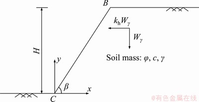
Figure 1 Sketch of problem statement

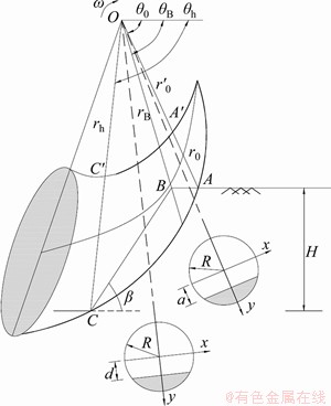
Figure 2 Longitudinal section of 3D rotational failure mechanism

3 3D rotational failure mechanism

To study the slope stability issues by using theoretical analysis methods, the slope failure mechanism must first be determined. Typical analysis of soil slope stability is on the basis of two-dimensional collapse models, e.g., the cylindrical failure model [7-9] and the log spiral failure model [5, 10]. However, recent studies showed that the practical slope collapse is three-dimensional (3D) failure, which indicates that the plane-strain (2D) failure mechanisms will inevitably lead to conservative estimations [11-14]. Therefore, by using 3D failure models, one can obtain more accurate prediction of slope stability, which could lead to significant savings in the construction of slopes [6]. In recent decades, some 3D collapse models, e.g., single block translational model [11], multi-block translational model [12], and 3D rotational model [13], are proposed to investigate the slope stability problem. In particular, the 3D rotational model is the most popular one [14]. To transform the 3D rotational model [13] into the plane-strain log spiral failure model, the 3D rotational model was modified by MICHALOWSKI et al [6] considering a “plane insert” by splitting and separating laterally the halves of 3D surface. Figure 2 shows the longitudinal section and cross section of the 3D rotational failure mechanism. Figure 3 shows the 3D rotational failure mechanism with plane-strain insert. Compared with other assumed models, the failure zone and stability numbers obtained by using the 3D rotational failure mechanism are more consistent with those from experiments and numerical simulations [15, 16].

Figure 3 3D rotational failure mechanism with plane-strain insert

As shown in Figure 3, it can be seen that the 3D rotational failure mechanism consists of two parts: the plane-strain insert and the 3D horn section. It is worth noting that b denotes the width of the plane-strain insert. When b→+∞, the 3D rotational failure mechanism will translate to the plane-insert mechanism.

The 3D horn section is the end part of the failure mechanism. As shown in Figure 2, the 3D rotational failure mechanism is bounded by two log-spirals in the longitudinal plane by respecting normality rule as follows [10]:

                           (1)

                          (2)

where r₀=OA and r₀'=O'A' (see Figure 2); φ is the frictional angle. In recent years, the 3D rotational failure mechanism has been widely used to estimate the stability of soil slopes by providing various stability number charts or critical seismic coefficient [15-18]. However, rare researches have studied the slope stability by giving the static FoS based on the 3D rotational failure mechanism. Moreover, little attention has been given to the relationship between the slope stability numbers and the critical seismic acceleration coefficient. This study will fill these research gaps.

4 Calculation of critical seismic acceleration coefficient

Because of the rigorous theoretical basis of the upper-bound limit analysis method, the stability assessment of slopes is conducted by using the upper-bound limit analysis method in this work. In the framework of the upper-bound limit analysis, the critical seismic acceleration coefficient is calculated by equating the total work rate of the energy dissipation to the total work rate of external forces as follows:

                            (3)

where D is the work rate of the energy dissipation; W_γ is the work rate of the soil weight; W_khis the work rate of the seismic load. The detailed derivation of the work rate of the energy dissipation and external forces can be described in the following subsections.

4.1 Work rate of internal energy dissipation

The work rate of the internal energy dissipation consists of two parts: the energy dissipation of the 3D horn section and the energy dissipation of the plane-strain insert. Therefore, the total work rate of the internal energy dissipation can be expressed as:

                          (4)

where D_3D and D_insert are the energy dissipation of the 3D horn section and the plane-strain insert, respectively. The energy dissipation of the 3D horn section D_3D can be calculated by:

(5)

with

                            (6)

                            (7)

where c is the soil cohesion; R is the radius of the cross section of the 3D rotational failure mechanism; a is the distance between the centreline of the conical volume and the crest surface AB; d is the distance between the centreline of the conical volume and the slope surface BC; w is the uniform angular velocity (see Figure 2); β is the slope angle (see Figure 3); θ₀, θ_B and θ_h respectively denote the values of angle between the line OA, OB and OC with the horizontal direction, as shown in Figure 2. The energy dissipation of the plane-strain insert D_insert can be described as:

 (8)

where b is the width of the plane-strain insert (see Figure 3).

4.2 Work rate of soil weight

As shown in Figure 3, it can be seen that the work rate of the soil weight consists of two parts: the work rate of the soil weight for the 3D horn section and the work rate of the soil weight for the plane-strain insert. Therefore, the total work rate of the soil weight can be calculated by:

                       (9)

where W_γ-3D and W_γ-insert are the work rate of the soil weight for the 3D horn section and the plane-strain insert, respectively. The work rate of the soil weight for the 3D horn section W_γ-3D can be expressed as:

          (10)

                           (11)

where r_m=(r+r')/2 and R=(r-r')/2. r and r' can be obtained in Eq. (1) and Eq. (2), respectively.

According to the geometrical relations, a and d can be obtained as:

                         (12)

             (13)

The work rate of the soil weight for the plane-strain insert W_γ-insert can be expressed by:

               (14)

with

       (15)

           (16)

           (17)

where L is the length of the plane-strain insert at the slope crest; r₀ is the length of OA; L/r₀ can be expressed as:

 (18)

4.3 Work rate of seismic loads

In this study, the seismic forces acting on the failure blocks are assumed to be uniform [19, 20]. Due to the fact that the vertical seismic acceleration has little influence on the slope stability [21], the vertical seismic acceleration is not considered in this study. It can be seen from Figure 3 that the work rate of the seismic loads can be divided into two parts: work rate of the seismic loads for the 3D horn section and work rate of the seismic loads for the plane-strain insert. The total work rate of the seismic load can be calculated by:

                     (19)

where W_kh-3D and W_kh-insert are the work rate of the seismic loads for the 3D horn section and the plane-strain insert, respectively. Combining Eq. (10) and Figure 3, the work rate of the seismic forces for the 3D horn section can be expressed as:

          (20)

where k_h is the horizontal seismic acceleration coefficient and can be calculated by:

                                (21)

where a_h is the horizontal seismic acceleration; g is the gravity acceleration. Combining Eq. (14) and Figure 3, the work rate of the seismic loads for the plane-strain insert section can be expressed by:

         (22)

with

(23)

           (24)

          (25)

where

4.4 Critical seismic acceleration coefficient

Combining Eq. (1) to Eq. (25), one can obtain the critical seismic acceleration coefficient by equating the total work rate of the energy dissipation to the total work rate of external forces in the framework of the upper-bound limit analysis theory as follows:

 (26)

The critical seismic acceleration coefficient k_hc obtained in this study is the minimum of Eq. (26) by employing all possible parameters θ₀, θ_h, r'₀/r₀, and b/H with given constraint soil parameters (φ, c, γ) and slope geometry (H, β). In this work, the algorithm of the particle swarm proposed by KENNEDY et al [22] is adopted for optimization.

5 Calculation of static FoS

In recent decades, various stability numbers have been proposed to estimate the slope stability [1-4, 23-26]. In the limit equilibrium method, the slope stability number is always defined as a function of the resisting force f_R divided by the driving force f_D [2]. While, in the limit analysis theory, the slope stability number is always defined as a function of the critical slope height H_cr, e.g., stability number N=c/γH_cr [3, 4]. Moreover, based on the finite element method, the static FoS is also widely adopted to analyze the slope stability issue by combining the strength reduction technique [1]. In this study, the static FoS of soil slopes is calculated to investigate the slope stability issue by using the 3D rotational failure mechanism. Based on the strength reduction technique, the static FoS is defined as the ratio of the actual soil shear strength to the minimum shear strength required to prevent failure as follows:

                      (27)

where c and j denote the natural soil cohesion and frictional angle, respectively; c_red and φ_red denote the reduced soil cohesion and frictional angle, respectively.

To calculate the static FoS of soil slopes in the upper-bound limit analysis, a coefficient SF is defined as:

                               (28)

where D and W_γ are work rates of energy dissipation and soil weight, and can be obtained by Eqs. (4) and (9), respectively. SF corresponds to the slope safety factor for each reduced material parameters. SF>1 implies that the slope is stable, which indicates that a larger FoS is needed to reduce the soil parameters (c and φ) to obtain the final static FoS. While SF<1 implies that the slope is unstable, which indicates that a smaller FoS is needed to reduce the soil parameters (c and φ) to obtain the final static FoS. To clearly describe the calculation of the static FoS of slopes based on the strength reduction technique, a computational flow is presented in Figure 4.

In Figure 4, FoS_min and FoS_max are the minimum and maximum factor of safety, respectively. It is worth noting that the initial FoS_min equals 0 and the initial FoS_max equals an appropriately large value within the range of precision and the consideration of calculation efficiency. The initial FoS equals 1. Figure 5 presents the static FoS based on the proposed method for the cases of B/H=5. From Figure 5, it can be seen that the static FoS increases with the increasing of the soil cohesion c and friction angle φ. From Figure 4, because of the additional iterative computations, the calculation of the static FoS needs more time for given slopes compared with the critical seismic acceleration coefficient. In this study, using the two processors of an E5-2667v3 8-core CPU 3.2QHz workstation, the calculation time of the static FoS is up to 3 min, while 3 s for the calculation of the critical seismic acceleration coefficient k_hc. Thus, if the calculated critical seismic acceleration coefficient can be used to determine the static FoS of slopes, then the amount of computation will be drastically reduced and valuable time will be saved.

Figure 4 Computation flow of static FoS

6 Results and discussion

In this section, the relationship between the static FoS and the critical seismic acceleration coefficient k_hc is presented. The analytical parameters are as follows: B/H=1, 2, 5, 10, φ= 5°-40°, β=45°-80°, and c/γH=0.05-0.25. The large amount of static FoS and k_hc from approximately 1000 slopes are plotted in Figure 6. From Figure 6, it can be seen that the calculated critical seismic acceleration coefficient k_hc increases with the increasing of static FoS. k_hc approximately equals 0 when FoS=1. By adopting a curve fitting strategy in MATLAB, a clear and strong relationship between static FoS and k_hc with the coefficient of determination R²=0.96 is obtained and plotted in Figure 6. The expression of the fitting formula can be described as:

             (29)

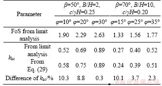
To validate the accuracy of Eq. (29), some comparisons between the critical seismic acceleration coefficient k_hc obtained by using the limit analysis method and those from Eq. (29) are shown in Table 1. From Table 1, it can be seen that the maximum discrepancy of the critical seismic acceleration coefficient k_hc obtained from the limit analysis and Eq. (29) is less than 10.5%, which indicates that Eq. (29) can be used to accurately estimate the critical seismic acceleration coefficient of slopes with given values of the static FoS.

Figure 5 Static FoS calculated based on proposed method when B/H=5 with:

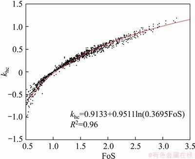
Figure 6 Critical seismic acceleration coefficient k_hc versus static FoS

Table 1 Comparison between the static FoS obtained from limit analysis method and Eq. (29)

To better validate the application of the proposed fitting formula, a practical slope case taken from DONALD [27] is presented. Its soil parameters are as follows: 1) c₁=0.001 kPa and φ₁=38° in soil layer 1; 2) c₂=5.3 kPa and φ₂=23° in soil layer 2; 3) c₃= 7.2 kPa and φ₃=20° in soil layer 3 (see Figure 7). The value of k_hc can refer to Ref. [23]. According to the existing k_hc=0.29 [23], the static FoS calculated from Eq. (29) is equal to 1.41. The static FoS from the finite element limit analysis (FELA) (OptumG2: version 2020) is equal to 1.42. And the difference between the static FoS form the proposed fitting formula (Eq. (29)) and numerical simulation is 0.7%. This indicates that the proposed fitting formula is also applicable to the complex practical slope.

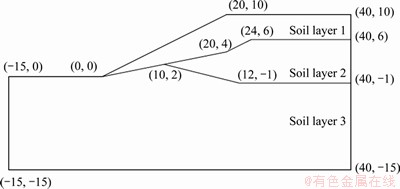
Figure 7 Schematic diagram of heterogeneous slope [27](Unit: m)

7 Conclusions

In this study, the relationship between the static FoS and the critical seismic acceleration coefficient k_hc of soil slopes is investigated based on the 3D rotational failure mechanism by using the upper-bound limit analysis. A fitting formula between the static FoS and k_hc is proposed in this study for the first time. Comparisons between the results from the proposed fitting formula with analytical and numerical results validate the accuracy of the proposed fitting formula.

A possible future research could be an extension of this work to determine the relationship between the static FoS and the earthquake-induced displacement of slopes by using the pseudo-dynamic method in heterogeneous and anisotropy soils.

Contributors

The overarching research goals were developed by SHI He-yang and CHEN Guang-hui. SHI He-yang edited the draft of manuscript and analyzed the calculated results. CHEN Guang-hui provided the concept and established the models. All authors replied reviewers’ comments and revised the final version.

Conflict of interest

SHI He-yang and CHEN Guang-hui declare that they have no conflict of interest.

References

[1] KRABBENHOFT K, LYAMIN A V. Strength reduction finite-element limit analysis [J]. Géotechnique Letters, 2015, 5(4): 250-253. DOI:10.1680/jgele.15.00110.

[2] SHEN Jia-yi, KARAKUS M, XU Chao-shui. Chart-based slope stability assessment using the generalized Hoek-Brown criterion [J]. International Journal of Rock Mechanics and Mining Sciences, 2013, 64: 210-219. DOI: 10.1016/ j.ijrmms.2013.09.002.

[3] SUN Zhi-bin, LI Jian-fei, PAN Qiu-jing, DIAS D, LI Shu-qin, HOU Chao-qun. Discrete kinematic mechanism for nonhomogeneous slopes and its application [J]. International Journal of Geomechanics, 2018, 18(12): 04018171. DOI: 10.1061/(asce)gm.1943-5622.0001303.

[4] KUMAR J, SAMUI P. Stability determination for layered soil slopes using the upper bound limit analysis [J]. Geotechnical & Geological Engineering, 2006, 24(6): 1803-1819. DOI: 10.1007/s10706-006-7172-1.

[5] HE Yi, LIU Yan, HAZARIKA H, YUAN Ran. Stability analysis of seismic slopes with tensile strength cut-off [J]. Computers and Geotechnics, 2019, 112: 245-256. DOI: 10.1016/j.compgeo.2019.04.029.

[6] MICHALOWSKI R L, DRESCHER A. Three-dimensional stability of slopes and excavations [J]. Géotechnique, 2009, 59(10): 839-850. DOI: 10.1680/geot.8.p.136.

[7] CHENG Y M, LANSIVAARA T, WEI W B. Two-dimensional slope stability analysis by limit equilibrium and strength reduction methods [J]. Computers and Geotechnics, 2007, 34(3): 137-150. DOI: 10.1016/ j.compgeo.2006.10.011.

[8] MAJUMDAR D K. Stability of soil slopes under horizontal earthquake force [J]. Géotechnique, 1971, 21(1): 84-88. DOI: 10.1680/geot.1971.21.1.84.

[9] SAHOO P P, SHUKLA S K. Taylor’s slope stability chart for combined effects of horizontal and vertical seismic coefficients [J]. Géotechnique, 2019, 69(4): 344-354. DOI: 10.1680/jgeot.17.p.222.

[10] CHEN W F. Limit analysis and soil plasticity [M]. Amsterdam: Elsevier, 2013.

[11] DRESCHER A. Limit plasticity approach to piping in bins [J]. Journal of Applied Mechanics, 1983, 50(3): 549-553. DOI: 10.1115/1.3167089.

[12] MICHALOWSKI R L. Three-dimensional analysis of locally loaded slopes [J]. Géotechnique, 1989, 39(1): 27-38. DOI: 10.1680/geot.1989.39.1.27.

[13] BALIGH M M, AZZOUZ A S. End effects on stability of cohesive slopes [J]. Journal of the Geotechnical Engineering Division, 1975, 101(11): 1105-1117. DOI: 10.1061/ajgeb6. 0000210.

[14] de BUHAN P, GARNIER D. Three dimensional bearing capacity analysis of a foundation near a slope [J]. Soils and Foundations, 1998, 38(3): 153-163. DOI: 10.3208/sandf. 38.3_153.

[15] YANG Xiao-li, XU Jing-shu. Three-dimensional stability of two-stage slope in inhomogeneous soils [J]. International Journal of Geomechanics, 2017, 17(7): 06016045. DOI: 10.1061/(asce)gm.1943-5622.0000867.

[16] NADUKURU S S, MICHALOWSKI R L. Three-dimensional displacement analysis of slopes subjected to seismic loads [J]. Canadian Geotechnical Journal, 2013, 50(6): 650-661. DOI: 10.1139/cgj-2012-0223.

[17] PAN Qiu-jing, XU Jing-shu, DIAS D. Three-dimensional stability of a slope subjected to seepage forces [J]. International Journal of Geomechanics, 2017, 17(8): 04017035. DOI: 10.1061/(asce)gm.1943-5622.0000913.

[18] HE Yi, HAZARIKA H, YASUFUKU N, HAN Zheng, LI Yan-ge. Three-dimensional limit analysis of seismic displacement of slope reinforced with piles [J]. Soil Dynamics and Earthquake Engineering, 2015, 77: 446-452. DOI: 10.1016/ j.soildyn.2015.06.015.

[19] SUN Chao-wei, CHAI Jun-rui, LUO Tao, XU Zeng-guang, MA Bin. Stability charts for pseudostatic stability analysis of rock slopes using the nonlinear Hoek-Brown strength reduction technique [J]. Advances in Civil Engineering, 2020, 3: 1-16. DOI: 10.1155/2020/8841090.

[20] SUN Chao-wei, CHAI Jun-rui, MA Bin, LUO Tao, GAO Ying, QIU Huan-feng. Stability charts for pseudostatic stability analysis of 3D homogeneous soil slopes using strength reduction finite element method [J]. Advances in Civil Engineering, 2019: 6025698. DOI: 10.1155/2019/ 6025698.

[21] GAZETAS G, GARINI E, ANASTASOPOULOS I, GEORGARAKOS T. Effects of near-fault ground shaking on sliding systems [J]. Journal of Geotechnical and Geoenvironmental Engineering, 2009, 135(12): 1906-1921. DOI: 10.1061/(asce)gt.1943-5606.0000174.

[22] KENNEDY J V, AUSTIN J, PACK R, CASS B. C-NNAP—A parallel processing architecture for binary neural networks [J]. Proceedings of ICNN’95-International Conference on Neural Networks, 1995, 2: 1037-1041. DOI: 10.1109/ICNN.1995. 487564.

[23] CHEN Guang-hui, ZOU Jin-feng, PAN Qiu-jing, QIAN Ze-hang, SHI He-yang. Earthquake-induced slope displacements in heterogeneous soils with tensile strength cut-off [J]. Computers and Geotechnics, 2020, 124: 103637. DOI: 10.1016/j.compgeo.2020.103637.

[24] SUN Chao-wei, CHAI Jun-rui, XU Zeng-guang, QIN Yuan, CHEN Xing-zhou. Stability charts for rock mass slopes based on the Hoek-Brown strength reduction technique [J]. Engineering Geology, 2016, 214: 94-106. DOI: 10.1016/ j.enggeo.2016.09.017.

[25] SUN Chao-wei, CHAI Jun-rui, XU Zeng-guang, QIN Yuan. 3D stability charts for convex and concave slopes in plan view with homogeneous soil based on the strength-reduction method [J]. International Journal of Geomechanics, 2017, 17(5): 06016034. DOI: 10.1061/(asce)gm.1943-5622.0000 809.

[26] WANG Yi-xuan, CHAI Jun-rui, CAO Jing, QIN Yuan, XU Zeng-guang, ZHANG Xian-wei. Effects of seepage on a three-layered slope and its stability analysis under rainfall conditions [J]. Natural Hazards, 2020, 102(3): 1269-1278. DOI: 10.1007/s11069-020-03966-1.

[27] DONALD I B, GIAM P. The ACADS slope stability programs review [C]// 6th International Symposium on Landslides, 1992, 3: 1665-1670.

(Edited by ZHENG Yu-tong)

中文导读

三维边坡临界地震加速度系数与静态安全系数的关系

摘要：现有的理论分析方法主要通过提供各种稳定性系数，例如静态安全系数或临界地震加速度系数实现对边坡稳定性的评估，而关于边坡安全系数与临界地震加速度系数的相关关系的研究较少。本文在极限分析上限分析法的框架下，探讨了三维边坡静态安全系数与临界地震加速度系数之间的关系。基于三维旋转破坏机理，首先，采用拟静力法给出了边坡临界地震加速度系数和采用强度折减技术给出了静态安全系数；然后，在考虑不同的坡角β、摩擦角φ和无量纲系数B/H和c/γH的条件下，研究了静态安全系数与临界地震加速度系数的相关关系；最后，给出了静态安全系数与临界地震加速度系数的拟合公式，并通过理论结果和数值结果对所提出的拟合公式进行了验证。

关键词：静态安全系数；临界地震加速度系数；极限分析上限分析法；三维旋转破坏机理

Foundation item: Project(2017YFB1201204) supported by the National Key R&D Program of China; Project(1053320190957) supported by the Fundamental Research Funds for the Central Universities, China

Received date: 2020-07-31; Accepted date: 2021-04-09

Corresponding author: CHEN Guang-hui, PhD Candidate; Tel: +86-15700731178; E-mail: guanghuichen@csu.edu.cn; ORCID: https://orcid.org/0000-0002-7051-4424