J. Cent. South Univ. Technol. (2010) 17: 1403-1408

DOI: 10.1007/s11771-010-0649-3

Theoretical solution of transient heat conduction problem in one-dimensional double-layer composite medium

ZHOU Long(周龙)^1,2, BAI Min-li(白敏丽)¹, L? Ji-zu(吕继组)¹, CUI Wen-zheng(崔文政)¹

1. School of Energy and Power Engineering, Dalian University of Technology, Dalian 116023, China;

2. School of Mechanical and Power Engineering, Henan Polytechnic University, Jiaozuo 454000, China

? Central South University Press and Springer-Verlag Berlin Heidelberg 2010

Abstract: To make heat conduction equation embody the essence of physical phenomenon under study, dimensionless factors were introduced and the transient heat conduction equation and its boundary conditions were transformed to dimensionless forms. Then, a theoretical solution model of transient heat conduction problem in one-dimensional double-layer composite medium was built utilizing the natural eigenfunction expansion method. In order to verify the validity of the model, the results of the above theoretical solution were compared with those of finite element method. The results by the two methods are in a good agreement. The maximum errors by the two methods appear when t (t is nondimensional time) equals 0.1 near the boundaries of ξ =1 (ξ is nondimensional space coordinate) and ξ =4. As t increases, the error decreases gradually, and when t =5 the results of both solutions have almost no change with the variation of coordinate ξ.

Key words: composite medium; transient heat conduction; theoretical solution; natural eigenfunction expansion method

1 Introduction

Heat conduction of composite medium is widely applied in many engineering and science areas, for instance, short pulse laser film heating [1], lens manufacturing [2], soil humidity [3], heat exchanger [4] and architectural design [5]. There are various research methods for solving transient heat conduction problem in composites, such as method of separation of variables [6], orthogonal expansion method [7], Laplace transform method [8], Green function method [9-11], Galerkin method [12-13] and integral-transform method [14]. However, among these methods, Laplace transform method only focuses on infinite or half-infinite objects, others return to the method of separation of variables in which thermal diffusivity is kept on the side of space variable function, and in essence, they are morbid.

Compared with other solving methods, natural eigenfunction expansion method makes the theoretical solution correspond to the nature of the studied phenomenon through putting thermal diffusivity on the side of time variable function. In addition, this method has the advantages of simple solving procedures of eigenvalue and eigenfunction and high efficiency. MONTE [15-16] solved transient heat conduction problems in one-dimensional double-layer and multi- layer composite media using natural eigenfunction expansion method. SUN and WICHMAN [17] investigated one-dimensional three-layer wall with fixed wall temperature by natural eigenfunction expansion method and the theoretical solution was extended to be suitable for arbitrary number of layers finally. However, both studies were based on the theoretical solution derivation of transient heat conduction equation and its boundary conditions that take the excess temperature as dependent variable utilizing natural eigenfunction expansion method. And then, the theoretical solution was transformed to the dimensionless form. The results of such processing made the theoretical solution model not a universal one and the equations deduced in the theoretical solution model very numerous and complicated, which greatly increased the complexity of the problem.

Thus, based on dimensionless treatment of relatively simple transient heat conduction partial differential equation and its boundary conditions using dimensionless factors and according to natural eigenfunction expansion method, a theoretical solution model for the problem of transient heat conduction in one-dimensional double-layer composite medium was developed. Utilizing the natural orthogonality relationship between eigenfunctions in the model established and adopting the method of graphics combining with numerical technique, a complete solution of transient heat conduction problem was obtained and verified by comparing with the solution of finite element method. Meanwhile, the positions near the boundaries where large errors appeared between two methods were further discussed.

2 Dimensionless treatment of heat conduction equation

As shown in Fig.1, a composite medium consisting of two parallel layers is considered, where, k₁ and k₂ are the thermal conductivities of the first and second layers, respectively; a₁ and a₂ are the thermal diffusivities; and x₁, x₂ and x₃ are the border coordinates. The two layers of the medium have initial temperatures of T₁(x) and T₂(x), respectively. At time t=0, two boundaries of the composite medium were heated by fluids with the same initial temperature T_f but different heat transfer coefficients of h₁ and h₂, separately.

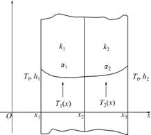
Fig.1 Sketch map of two-layer composite medium

Assume that perfect thermal contact conditions are satisfied, and thermal conductivity and thermal diffusivity are fixed within each layer. T₀ represents the same temperature of the composite region, and T₁ and T₂ are temperatures of the two layers, respectively.

The following dimensionless factors are introduced in order to transform one-dimensional transient heat conduction partial differential equation and its boundary conditions to dimensionless forms:

(i=1, 2), and (i=1, 2, 3).

where ξ is the nondimensional space coordinate; τ is the nondimensional time; B_i is the Biot number; κ is the thermal conductivity ratio; δ is the thermal diffusion ratio; Θ is the nondimensional temperature; and γ is the nondimensional interface coordinate. Subscript i represents the first and the second layers or the interface position.

One-dimensional transient heat conduction partial differential equation can be written as follows (τ≥0):

                              (1)

where  i=1, 2.

Outer boundary conditions become:

             (2)

Inner boundary conditions become ():

                      (3)

Initial conditions become:

                       (4)

where i=1, 2; and represents the initial temperature of the ith layer transformed from T_i(x).

3 Solving of dimensionless heat conduction equation

Using method of separation of variables to solve Eq.(1), we have

                        (5)

where τ≥0;  i=1, 2; X_i(ξ) represents the spatial variable function; and G_i(τ) is the time variable function.

Introducing Eq.(5) into Eq.(1) and using natural eigenfunction expansion method, separate equations of functions G_i(τ) and X_i(ξ) can be derived:

                             (6)

where τ≥0, and i=1, 2.

                             (7)

where i=1, 2; and l_i is the separation constant corresponding to the ith layer of the composite medium.

The solutions of G_i(τ) and X_i(ξ) can be gained by solving Eqs.(6)-(7).

                               (8)

where τ≥0, and i=1, 2.

                 (9)

where  i=1, 2; and a_i and b_i are integral constants corresponding to the ith layer of the composite medium.

3.1 Application of boundary conditions

Introducing Eq.(5) into Eqs.(2)-(3), supposing λ₁=λ (l is an arbitrary number greater than zero), a₁=c (c is a constant dependent on initial conditions (4)), and using δ₁=1, solution of  (i=1, 2) can be written as:

                (10)

wherei=1, 2; and are defined as

                          (11)

Function  (i=1, 2) may be written as

     (12)

wherei=1, 2.

Function (i=1, 2) is given by

           (13a)

          (13b)

whereis the derivative of

Introducing Eq.(5) into boundary condition of  and comparing with Eq.(13b), we have

   (14)

Thus, Eq.(14) is the equation of computing eigenvalues.

Eq.(10) satisfies Eqs.(1)-(3). Thus, Eq.(10) has an infinite number of solutions and each corresponds to a series of eigenvalues λ₁＜λ₂＜…＜λ_m＜… (m=1, 2, 3, …):

               (15)

where τ≥0; i=1, 2; and

Function(i=1, 2) is the eigenfunction corresponding to eigenvalue λ_m.

    (16)

where and i=1, 2.

It is very easy to prove that the eigenfunctions (i=1, 2) satisfy the following orthogonal relationship:

(17)

where functionsandrepresent different eigenfunctions corresponding to eigenvalues λ_m and λ_n respectively in the ith layer; and the solving of constant N_m can be found in Ref.[15].

The solution of temperature distribution  (i=1, 2) is composed of the fundamental solutions of the above separated equations according to the principle of linear superposition:

              (18)

where τ≥0; and i=1, 2.

3.2 Application of initial conditions

Introducing initial conditions (4) into Eq.(18) yields:

               (19)

where τ≥0;and i=1, 2.

Multiplying both sides of Eq.(19) by operator  according to Eq.(17), coefficient c_m is

            (20)

where the solution of the integration on the right side of Eq.(20) can be found in Ref.[15].

4 Example analysis and numerical verifica- tion

The following values to the defined dimensionless parameters are employed: γ₁=1, γ₂=2, γ₃=4, κ₁=1, κ₂=2, δ₁=1, δ₂=1,

4.1 Determination of eigenvalues

The first step for the solution of Eq.(15) concerns the determination of the eigenvalues. In this case, it is not possible to obtain an explicit solution from Eq.(14) for eigenvalue λ. However, the problem can be solved by means of the combination of both a graphical and a numerical scheme. Hence, two functions Π₁₁(λ) and Π₂₂(λ) are used to express Eq.(14), that is, Π₁₁(λ)= Π₂₂(λ).

The changes of functions Π₁₁(λ) and Π₂₂(λ) against λ are shown in Fig.2. The asymptotes of functions Π₁₁(λ) and Π₂₂(λ) can also be seen in the figure. The intervals that Eq.(14) have roots can be determined utilizing the asymptotes of function Π₂₂(λ). For each inter-district, root λ of Eq.(14) can be obtained by means of Newton iteration procedure, as shown in Table 1.

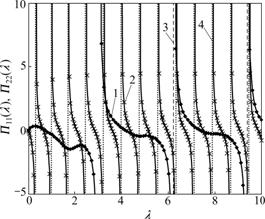
Fig.2 Changes of functions Π₁₁(λ) and Π₂₂(λ) against λ: 1—Π₁(λ); 2—Π₂₂(λ); 3—Vertical asympototes of Π₁₁(λ); 4—Vertical asymptotes of Π₂₂(λ)

4.2 Determination of amount of eigenvalues p

After the determination of eigenvalues, the second step is to determine the amount of eigenvalues p. For general engineering problems, p can be determined by requiring that the exact (p→∞) and approximate (p= finite) solutions are differed by not more than 3%. For space coordinate ξ, the maximum deviations of  (i=1, 2) between the exact (p→∞) and approximate (p=finite) solutions occur near the outer boundary surfaces that can be observed in Fig.3. In order to achieve the same convergence accuracy, more eigenvalues should be solved on the outer boundary surfaces. That is, more summing calculations of function terms need to be done. And for time coordinate τ, the maximum deviations appear at τ= 0. Therefore, positions ξ=1 and ξ=4 and time τ=0 are the best positions and time to determine the amount of eigenvalues p.

Fig.3 shows the changes of dimensionless temperature(i=1, 2) with different values of parameter p against coordinate ξ for τ=0. Fig.3 shows that functions (i=1, 2) are continually approximating towards a definite limit when increasing the amount of eigenvalues p. When taking a limiting process (p→∞), functions  (i=1, 2) converge to 1. When taking p=23, the error of the exact (p→∞) and approximate (p=finite) solutions is less than 2.6% for ξ=γ₁, and less than 2.7% for ξ=γ₃. Although for sufficiently large time τ, p can be notably reduced. In order to reduce the error, p=23 is fixed when requiring the approximate solutions of (i=1, 2) at time τ.

Table 1 First 25 roots of transcendental Eq.(14)

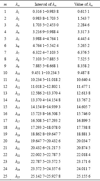
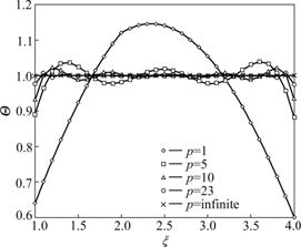
Fig.3 Dimensionless temperature  for τ=0 as function of ξ with p as parameter (interface is located at x=2)

4.3 Numerical verification

Fig.4 shows the comparison of solving by natural eigenfunction expansion and finite element methods. As shown in Fig.4(a), the results of both methods are coinciding, which shows that the solutions of two methods are kept consistent with each other. The maximum errors occur at boundaries of x＝1 and x＝4 when t＝0.1. The finite element solutions are 0.039 and 0.051 larger than theoretical solutions, respectively. The reason is that Eq.(18) needs to calculate more eigenvalues λ at the outer boundaries to achieve higher accuracy, however, the cost is extra computational time. And in the solving, in order to govern the error between exact (p→∞) and approximate solutions (p=finite) to be less than 3%, only the first 23 eigenvalues were used. And in Fig.4(b), when t is small, the error between finite element and theoretical solutions changes significantly against the change of coordinate ξ. The maximum errors occur at boundaries x＝1 and x＝4 when t＝0.1, which are 3.91% and 5.08%, respectively. At the other moments and positions, the error is lower than 1%. With the increase of t, the error between two methods varying against the change of coordinate ξ becomes less. When  t＝5, two solutions remain unchanged against the change of coordinate ξ.

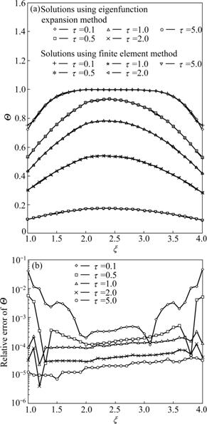
Fig.4 Comparison of solutions using natural eigenfunction expansion and finite element methods (interface is located at x=2): (a) Dimensionless temperature; (b) Relative error at each point x and specified time t

5 Conclusions

(1) Firstly, the transient heat conduction model is transformed to the dimensionless form. Then, the dimensionless thermal diffusivity is put on the side of time variable function. Thus, the physical essential of the phenomenon can be embodied by transformed equation of heat conduction. A theory solution model of transient heat conduction problem in one-dimensional double- layer composite medium is developed. The model is more generic compared with those in Refs.[15-17], and steps of derivation and expressions are much simpler.

(2) A method that combines graphics and numerical methods is adopted and Newton iterative method is used in each small interval for calculating eigenvalues. The eigenvalues model developed is calculated, and the problem unable to calculate eigenvalue equation using numerical method alone is solved.

(3) Validity and rationality of the theory solution model are validated by finite element method. At time   τ＝0, the maximum errors occur at boundaries of ξ=1 and ξ=4. And the smaller the time τ, the larger the error. Through calculating Eq.(14) with more eigenvalues λ and increasing the summation items in Eq.(18), the error can be decreased efficiently. However, the cost consumes much more computing time.

References

[1] WANG H J, DAI W Z, LIONEL G H. A finite difference method for studying thermal deformation in a double-layered thin film with imperfect interfacial contact exposed to ultrashort pulsed lasers [J]. International Journal of Thermal Science, 2008, 47: 7-24.

[2] YIN H, WANG L, FELICELLI S D. Comparison of two-dimensional and three-dimensional thermal models of the LENS process [J]. Journal of Heat Transfer, 2008, 130: 1-7.

[3] GE X Y, MIKI W, YAN G G. Analytical solutions for time-dependent heat conduction equation of soil moisture [J]. Nonlinear Analysis: Real World Applications, 2009, 10: 1923-1931.

[4] GANDJALIKHAN S A, MARAMISARAN M. Transient numerical analysis of a multi-layered porous heat exchanger including gas radiation effects [J]. International Journal of Thermal Sciences, 2009, 48: 1586-1595.

[5] L? X, LU T, VILJANEN M. A new analytical method to simulate heat transfer process in buildings [J]. Applied Thermal Engineering, 2006, 26: 1901-1909.

[6] VODICKA V. W?rmeleitung in geschichteten kugel- undzylinderk?rpen[M]. Schweiz: Arch Press, 1950: 297-304.

[7] MIKHAILOV M D, ?ZISIK M N, VULCHANOV N L. Diffusion in composite layers with automatic solution of the eigenvalue problem [J]. International Journal of Heat and Mass Transfer, 1983, 26: 1131-1141.

[8] CARSLAW H S, JAEGER J C. Conduction of heat in solids [M]. London: Oxford University Press, 1959: 218-235.

[9] HUANG S C, CHANG Y P. Heat transfer in unsteady periodic and steady states in laminated composites [J]. Journal of Heat Transfer, 1980, 102: 742-748.

[10] FENG Z G., MICHAELIDES E E. The use of modified Green’s functions in unsteady heat transfer [J]. International Journal of Heat and Mass Transfer, 1997, 40: 2997-3002.

[11] SIEGEL R. Transient thermal analysis of parallel translucent layers by using Green’s functions [J]. Journal of Thermophysics and Heat Transfer, 1999, 13(1): 10-17.

[12] HAJISHEIKH A, BECK J V. Green’s functions partitioning in Galerkin-based integral solution of the diffusion equation [J]. Journal of Heat Transfer, 1990, 112: 28-34.

[13] HEIDEMANN W, MANDEL H, HAHNE E. Computer aided determination of closed form solutions for linear transient heat conduction problems in inhomogeneous bodies [J]. Transactions on Engineering Sciences, 1994, 5: 19-26.

[14] YENER Y, ?ZISIK M N. On the solution of unsteady heat conduction in multi-region finite media with time-dependent heat transfer coefficient [C]// Proceedings of the Fifth International Heat Transfer Conference. Tokyo: JSME, 1974: 188-192.

[15] MONTE F D. Transient heat conduction in one-dimensional composite slab: A ‘natural’ analytic approach [J]. International Journal of Heat and Mass Transfer, 2000, 43: 3607-3619.

[16] MONTE F D. An analytic approach to the unsteady heat conduction processes in one-dimensional composite media [J]. International Journal of Heat and Mass Transfer, 2002, 45: 1333-1343.

[17] SUN Y Z, WICHMAN I S. On transient heat conduction in a one-dimensional composite slab [J]. International Journal of Heat and Mass Transfer, 2004, 47: 1555-1559.

(Edited by CHEN Wei-ping)

Corresponding author: BAI Min-li, Professor; Tel: +86-411-84706305; E-mail: baiminli@dlut.edu.cn