J. Cent. South Univ. (2016) 23: 2858-2866

DOI: 10.1007/s11771-016-3349-9

Bayesian zero-failure reliability modeling and assessment method for multiple numerical control (NC) machine tools

KAN Ying-nan(阚英男)¹, YANG Zhao-jun(杨兆军)¹, LI Guo-fa(李国发)¹, HE Jia-long(何佳龙)¹,

WANG Yan-kun(王彦鹍)¹, LI Hong-zhou(李洪洲)^{1, 2}

1. College of Mechanical Science and Engineering, Jilin University, Changchun 130025, China;

2. College of Mechanical Engineering, Beihua University, Jilin 132011, China

Central South University Press and Springer-Verlag Berlin Heidelberg 2016

Abstract: A new problem that classical statistical methods are incapable of solving is reliability modeling and assessment when multiple numerical control machine tools (NCMTs) reveal zero failures after a reliability test. Thus, the zero-failure data form and corresponding Bayesian model are developed to solve the zero-failure problem of NCMTs, for which no previous suitable statistical model has been developed. An expert-judgment process that incorporates prior information is presented to solve the difficulty in obtaining reliable prior distributions of Weibull parameters. The equations for the posterior distribution of the parameter vector and the Markov chain Monte Carlo (MCMC) algorithm are derived to solve the difficulty of calculating high-dimensional integration and to obtain parameter estimators. The proposed method is applied to a real case; a corresponding programming code and trick are developed to implement an MCMC simulation in WinBUGS, and a mean time between failures (MTBF) of 1057.9 h is obtained. Given its ability to combine expert judgment, prior information, and data, the proposed reliability modeling and assessment method under the zero failure of NCMTs is validated.

Key words: Weibull distribution; reliability modeling; Bayes; zero failure; numerical control (NC) machine tools; Markov chain Monte Carlo (MCMC) algorithm

1 Introduction

1.1 Zero-failure problem of multiple numerical control machine tools (NCMTs)

NCMTs, which are the basic equipment for advanced manufacturing, consist of mechanical, electronic, hydraulic parts and so on and belong to a complex repairable system. Their reliability is of significant importance because their breakdown may mean a cessation of the production line [1]. In practice, almost all reliability tests on entire systems of NCMTs are field tests at users [2]. A field test always requires a large amount of time and many NCMTs to obtain sufficient data and implement reliability modeling and assessment using classical statistical methods. For example, KELLER et al [3] conducted a field test on 35 NCMTs over three years and dealt with data using least squares estimation (LSE) and maximum likelihood estimation (MLE). JIA et al [4] conducted a field test on 24 NCMTs for about one year and dealt with data using LSE. YANG et al [5] conducted a field test on 12 NCMTs for about five years and dealt with data using MLE.

However, the reliability level (RL) of NCMTs is improved as the technology improves. The number of available tested NCMTs is decreasing because the NCMT products of one model are usually produced in a small lot at present, and the test time cannot be extended any more given that the update of NCMT products is accelerating. Given the above reasons, the number of failures in a test is currently decreasing dramatically. Moreover, several reliability tests on multiple NCMTs have actually revealed zero failures. Thus, a new problem of reliability modeling and assessment under zero-failure data arises, which is called the zero-failure problem. The zero-failure problem cannot be solved by classical statistical methods, which rely on a large number of failures, such as LSE and MLE. Therefore, developing a solution to the zero-failure problem of multiple NCMTs is of significance. Existing methods for zero-failure data are reviewed first below.

1.2 Existing methods for zero-failure data

Existing methods for zero-failure data mainly fall into two categories: reliability demonstration test (RDT) and reliability modeling and assessment. In RDT, a zero-failure result is common and is usually taken as a proof to demonstrate that the pre-specified reliability target has been reached. By contrast, research on reliability modeling and assessment under zero failures is scanty. The literature on both categories is reviewed in what follows.

The earliest work on zero-failure RDT was accomplished by MARTZ and WALLER using a Bayesian method [6], where the failure time of a component of a nuclear reactor safety system is assumed to follow an exponential distribution and a gamma prior distribution is adopted for the failure rate. The posterior distribution is derived when the number of failures is zero. Given a posterior risk criterion, the combination of number of products, n, and test time, t, is obtained, according to which the test plan is designed. In the example [6], if the test reveals zero failures given n×t=1987 (unit: h), the pre-specified RL is demonstrated. COOLEN et al [7-8] studied the zero-failure RDT for a system’s (e.g., alarm system) tasks using Bayesian methods, where the number of tasks follows a Poisson distribution. FAN and CHANG [9] proposed a Bayesian zero-failure RDT plan for electro-explosive devices, whose lifetime follows an exponential distribution. YANG [10] proposed a zero-failure RDT plan for electromagnetic valves using degradation data.

With respect to reliability modeling and assessment, MAO and XIA [11] proposed a Bayesian estimation method for the zero-failure result of a reliability test on engines. This method requires n products to be divided into k groups, and the number of products in each group is denoted by n_i, i=1, 2, …, k. Respective time-censored tests are conducted on each group, where the testing time is denoted by t_i, i=1, 2, …, k, and t₁2<…k. If zero failures are observed, then the zero-failure data are denoted by (t_i, n_i). This method requires a point estimator of the cumulated failure probability, P_i, at each t_i by experts, and a Weibull curve is fitted through the points (t_i, P_i) using LSE to obtain the estimators of the Weibull parameters. HAN and DING [12] proposed an E-Bayesian method for an exponential distribution under zero-failure data, and the test plan is similar to that of MAO and XIA [11]. JIANG et al [13] used Weibull distribution to solve zero-failure estimation, which improved the calculation techniques of the Bayesian methods, compared to the method proposed by MAO and XIA [11]. JIANG et al [14] proposed a modified MLE for Weibull distribution under zero-failure data. MILLER et al [15] developed a formula to calculate the failure probability of software under zero failures based on Bayesian methods. XU and CHEN [16] proposed a Bayesian method to estimate the two-sided credible limits of exponential parameters under zero failures. GUO et al [17] combined the Bayesian methods and classical methods to present a formula to calculate the success rate of rockets or missiles, where the success number follows a binomial distribution.

1.3 Solution to zero-failure problem of NCMTs

The literature reviewed above basically represents the current status of reliability research relevant to zero-failure data. However, most of these studies are aimed at specific types of products, such as components of nuclear reactor safety systems, a fire alarm system in a plant, electro-explosive devices, electromagnetic valves, engines, software, missiles, and rockets. Thus, none of the above methods is suitable for NCMTs for the following reasons.

1) The two-parameter Weibull distribution is widely accepted as the most suitable model that describes the time between failures (TBF) of NCMTs by many scholars in the machine tools industry, such as KELLER et al [3] and JIA et al [4]. Thus, the methods aimed at zero-failure data that are based on exponential [6, 9, 12, 16], Poisson [7-8], or binomial [15, 17] distributions are not suitable for NCMTs.

2) The methods that deal with zero failures using degradation data are always aimed at a part or a component, whereas an NCMT is a complex system. Thus, a method aimed at zero failures using degradation data [10] is not suitable for NCMTs.

3) Although Refs. [11, 13-14] are aimed at Weibull distribution under zero failures, the test plans require the following items: (1) The number of tested products ought to be large enough. (2) The tested products ought to be divided into k groups, and k is supposed to be larger than 10 to guarantee the accuracy. (3) The test time for each group ought to be different. These requirements are infeasible for NCMTs for the following reasons: (1) The above test plans are suitable for laboratory tests or components, but a test on NCMTs must be a field test on entire, complex systems in a manufacturing company under real working and loading conditions. (2) A company cannot provide many NCMTs of the same model in one site. (3) Designing various time-censored tests is impossible, given that tests should not interrupt the normal operation of a manufacturing company, and the test time for NCMTs is always a single, fixed value [3-4].

In conclusion, (1) none of the above methods is suitable for the zero-failure problem of multiple NCMTs, and (2) nearly all the solutions to zero-failure data are Bayesian methods, which exhibit great advantages over classical statistical methods. Given that no previous study has paid attention to NCMTs, the proposal of a Bayesian method of reliability modeling and assessment aimed at zero-failure data for multiple NCMTs is innovative and of great significance.

A complete Bayesian method that solves the zero-failure problem of multiple NCMTs largely consists of the following three stages:

1) Given that no previous, suitable statistical model exists to describe the zero-failure problem of NCMTs, a corresponding Bayesian model needs to be developed, including descriptions of TBF, form of zero-failure data, and the prior and posterior distributions of the Weibull parameters.

2) Expert judgment is important in Bayesian methods to build the prior distributions of parameters [18-19]. The direct presentation of the prior distributions of the Weibull parameters is difficult, whereas the presentation of the prior distribution of the Weibull cumulative distribution function (CDF) is comparatively easier [20]. As such, an indirect process that consists of two stages is proposed. The first stage is to combine expert judgment with prior information to obtain the estimated intervals of the Weibull CDF values at two time points. The second stage is to transform the CDF intervals into the prior distributions of the Weibull parameters.

3) The calculation of the posterior distributions of the Weibull parameters involves a high-dimensional integration that cannot be solved analytically. Thus, further analytical solutions to the parameter estimators and the mean time between failures (MTBF) are impossible, and a numerical method is needed. The development of an MCMC simulation algorithm will solve the above difficulties.

4) A real-case application is provided and the details of running an MCMC simulation in the software WinBUGS are presented.

2 Bayesian zero-failure model for multiple NCMTs

2.1 Two-parameter Weibull distribution

The two-parameter Weibull distribution is adopted to describe the TBF of NCMTs according to tradition [3-4]. The CDF and reliability function are given by Eqs. (1) and (2):

              (1)

               (2)

where the random variable T denotes TBF; F(t|α,β) represents the probability that T≤t; R(t|α,β) represents the probability that T>t; t is time; α is the scale parameter, which is larger than 0; β is the shape parameter, which is larger than 0; the parameter vector is denoted by θ=(α, β). In addition, the intuitive assumption that α and β are independent of each other is adopted, since no study and information are available to show any relation between the two parameters.

2.2 Denoting prior distributions of Weibull parameters

From the perspective of Bayesian statistics, the Weibull parameters are random variables that have their own distributions called prior distributions, which exist before and independent of the data. Here, π(α) and π(β) are two probability density functions (PDF), which denote the prior distributions of α and β, respectively; and π(θ) denotes the prior distribution of θ. Thus, π(θ) is provided by Eq. (3):

                    (3)

2.3 Zero-failure data for multiple NCMTs

The number of tested NCMTs of the same model is denoted by n, and each NCMT is indexed by i=1, 2, …, n. The test time and TBF for the ith NCMT are denoted by τ_i and T_i, respectively. Thus, the zero-failure event for the ith NCMT is a censored datum expressed by T_i>τ_i. The corresponding zero-failure data sample for n NCMTs is denoted by τ={τ_i}, where i=1, 2, …, n. The probability of T_i>τ_i is denoted by P(T_i>τ_i|θ), which is calculated by substituting τ_i into the reliability function, Eq. (2), as shown in Eq. (4):

    (4)

The value of Eq. (4) is also called the likelihood contribution of τ_i. According to the multiplication principle, the complete likelihood function of the data sample τ={τ_i} is given by

          (5)

2.4 Posterior distributions of parameters

The prior distribution of the parameter vector θ is updated into a posterior distribution in light of the data sample τ. The posterior distribution is obtained via Bayes theorem. A general form of Bayes theorem is given by

                        (6)

where P(τ) is the marginal distribution of the data sample τ={τ_i}, which is calculated by

          (7)

where the value of P(τ) is a constant, after the integration of the parameters.

Substituting Eqs. (3), (5) and (7) into Eq. (6) obtains the theoretical formula for the posterior distribution of θ:

     (8)

The posterior distributions of α and β, denoted by π(α|τ) and π(β|τ), can be derived from π(θ|τ). The parameter estimations for α and β are based on π(α|τ) and π(β|τ), respectively.

As discussed in Section 1.3, the Bayesian model for the zero-failure problem of NCMTs is established by Eqs. (1)–(8).

3 Building prior distributions of parameters

3.1 Expert-judgment process

Suppose that A and B are two models of NCMT. The RLs of A and B are denoted by RL(A) and RL(B), respectively, and the MTBFs of A and B are denoted by MTBF(A) and MTBF(B), respectively. Although experts may be unfamiliar with the probability or reliability knowledge, they can judge whether RL(A) is higher or lower than RL(B) qualitatively by comparing the common attributes of the NCMTs. These attributes include: the technology level of an NCMT’s manufacturer, cost of an NCMT, complexity of an NCMT’s structure, degree of diversity of an NCMT’s functions, and degree of satisfaction of an NCMT’s user. The information on these attributes is called multi-source prior information.

Based on engineering experience and experts’ opinions in the NCMT industry, an assumption is concluded and presented as follows: If the RL(A) is higher than the RL(B) qualitatively, then the MTBF(A) is larger than the MTBF(B) quantitatively. This assumption is called the RL-MTBF assumption.

Given the above discussion and assumption, the expert-judgment process is proposed as follows:

1) The tested model of NCMT is denoted by M, and multi-source prior information on M should be collected by the facilitators [18] (or assessors [19]), who are responsible for leading the whole expert-judgment process. At least two facilitators are required: one should have a deep knowledge of reliability theory, and the other should be a manager from the company where the test takes place.

2) The facilitators identify the expert panel, which consists of at least one NCMT designer, one service engineer, one quality engineer, one sales engineer, one maintenance worker, and one machine operator. The number of experts is denoted by p, and each expert is denoted by E_j, j=1, 2, …, p.

3) The expert panel identifies several models of NCMT, which are similar to M and have sufficient historical data. The number of identified models is q, and they form a set S={S₁, S₂, …, S_k, …, S_q}, where each element S_k denotes a model of NCMT and k=1, 2, …, q. The TBF model and MTBF of each S_k is available based on classical statistical methods and its historical data. The facilitators should first arrange the elements of S in ascending order of MTBF to form a standard permutation (SP):

               (9)

where MTBF(S_(k))< MTBF(S_(k+1)), k=1, 2, …, q-1.

4) The multi-source prior information on {S₁, S₂, …, S_k, …, S_q} should be collected by the facilitators and experts.

5) Without knowing the SP and MTBFs of S₁, S₂, …, S_q, each expert E_j is required to receive and process the prior information and then sort S₁, S₂, …, S_q in ascending order of RLs, forming a permutation named permutation PE_j:

       (10)

where expert E_j believes j=1, 2, …, p; k=1, 2, …, q-1.

Given that expert E_j does not know SP, PE_j may not be identical to SP. Thus, a practice process is needed, where facilitators should remind each expert E_j to practice and adjust PE_j many times, until PE_j is identical to SP. Expert E_j is then believed to be qualified to give reliable judgment for the next step.

6) The experts are asked to insert M between two elements of SP. A final consensus among the experts is required after their communication and discussion to form the final permutation (FP):

        (11)

where RL(S_(k))(k+1)); k=1, 2, …, q-1.

The above six steps are illustrated by a flow chart in Fig. 1.

3.2 Distribution intervals for CDF values

In FP, S_(k) and S_(k+1) are denoted by M- and M+, respectively. Two appropriate time points t₁ and t₂ are selected. Given that the historical TBF distributions of M- and M+ are available, their CDF values at t₁ and t₂ are calculated by Eq. (1) and denoted by P_M-,1, P_M-,2, P_M+,1, and P_M+,2. Based on engineering experience, an NCMT with a higher RL is assumed to have a smaller CDF value at an appropriate time point. Thus, the following relation is obtained: P_M+,1< P_{M-, 1} and P_M+,2

M_{-, 2} (see Fig. 2).

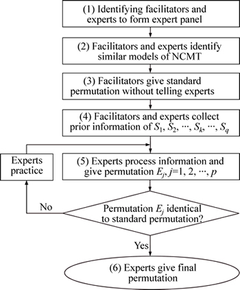
Fig. 1 Flow chart of expert-judgment process

For M, the CDF values at t₁ and t₂ are denoted by P₁ and P₂, respectively. The distribution intervals for P₁ and P₂ are denoted by (P_1L, P_1U) and (P_2L, P_2U), respectively, where (P_1L, P_1U)=(P_{M+, 1}, P_{M-, 1}) and (P_2L, P_2U)=(P_{M+, 2}, P_{M-, 2}) (see Fig. 2).

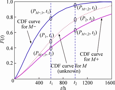
Fig. 2 Illustrative CDF curves for M-, M and M+

3.3 Building prior distributions of parameters

Based on the method proposed by KAMINSKIY and KRIVTSOV [20], the intervals (P_1L, P_1U) and (P_2L, P_2U) can be transformed equivalently into the distribution intervals of the Weibull parameters: (α_L, α_U) and (β_L, β_U). The transformation process is as follows:

First, according to Eq. (1), two equations can be obtained:

             (12)

            (13)

Based on Eqs. (12) and (13), β and α are derived, respectively:

             (14)

              (15)

Given the fixed t₁ and t₂, β and α are treated as two functions of (P₁, P₂), which are provided by Eqs. (14) and (15), respectively. P₂ is larger than P₁, because the CDF is monotonically increasing. The function plots of α(P₁, P₂) and β(P₁, P₂) are given in Figs. 3 and 4, under P₂> P₁, respectively.

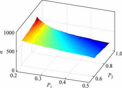
Fig. 3 Plot of function α(P₁, P₂)

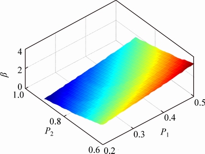
Fig. 4 Plot of function β(P₁, P₂)

The function plots show that the combinations of the extreme values of P₁ and P₂ determine the extreme values of α or β. Thus, if (P_1L, P_2L), (P_1L, P_2U), (P_1U, P_2L), and (P_1U, P_2U) are substituted into Eqs. (14) and (15), respectively, then the maximum and minimum values of α and β can be obtained from the results, which are denoted by α_L, α_U, β_L, and β_U. Given that no further information is available, the uniform distributions are assumed on (α_L, α_U) and (β_L, β_U), respectively, following BERGER’s work [21]. Thus, the prior distributions of α and β are given by the following two PDFs:

             (16)

              (17)

4 MCMC simulation and WinBUGS

The P(τ) in Eq. (7) or the denominator on the right side of Eq. (8) is a high-dimensional integration, given that two unknown random variables, α and β, exist, and the integrated function is complex. Thus, Eq. (8), the theoretical formula for the posterior distribution of θ, does not have a closed form [20], and analytic solutions for further parameter estimations are unavailable. Thus, to solve high-dimensional integration and parameter estimations, an MCMC algorithm is needed.

Although P(τ) cannot be solved analytically, it is a constant [20]. Thus, Eq. (8) is rewritten in a proportional form:

           (18)

where Eq. (18) is the basis for developing an MCMC algorithm to simulate the posterior distributions, π(α|τ) and π(β|τ).

The MCMC simulation algorithms include the Gibbs sampler, Metropolis–Hastings algorithm, slice sampling, and others [22-23]. The task of an MCMC algorithm is to draw samples from the posterior distribution of a parameter to form a Markov chain. When the Markov chain reaches its static distribution, the samples can be seen as drawn from the target posterior distribution; thus, the sample statistics can approximate the theoretical statistics [22]. Although developing an MCMC algorithm manually is challenging for general practitioners, many tools have been developed to assist them. The most famous one may be the free software package WinBUGS.

WinBUGS can run various MCMC algorithms. Many scholars, such as WANG et al [24], use WinBUGS to implement MCMC algorithms. In WinBUGS, any Bayesian problem should first be described in a language called BUGS to build a BUGS model. A BUGS model mainly consists of four parts: (1) description of the prior distributions of the parameters, (2) description of the likelihood function, (3) description of data, and (4) initial values of the parameters to be simulated. The expert system on WinBUGS can select a specific MCMC algorithm suitable for the Bayesian problem according to the BUGS model [25]. Generally, WinBUGS selects slice sampling [23] to solve a complex problem. The detailed operation of WinBUGS for the zero-failure problem of NCMTs is illustrated in a real-case application in Section 5.

5 Real-case application

5.1 Zero-failure data

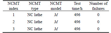
A field reliability test was implemented on three NCMTs of the same model M. The testers were from our college, and the tested three NCMTs were located at the workshop of a manufacturing company. The test was started when the testers arrived and finished when the testers left. The test time was 496 h, and all the three NCMTs were operated without failure throughout the test. Zero failures were observed, and the corresponding data are given in Table 1.

Table 1 Zero-failure data of three tested NCMTs

5.2 Process of expert judgment

According to Section 3.1, the expert-judgment process was implemented as follows:

1) A professor familiar with the reliability knowledge of NCMTs and a manager from the manufacturing company where the test took place served as two facilitators.

2) The facilitators identified the expert panel consisting of six experts E_j (j=1, 2, …, 6).

3) The expert panel identified five models of NCMT similar to M and formed a set S={S₁, S₂, S₃, S₄, S₅}. The TBF model and MTBF of each S_k were obtained by the facilitators based on LSE and sufficient historical data. SP={S₍₁₎, S₍₂₎, S₍₃₎, S₍₄₎, S₍₅₎} was then obtained, where MTBF(S_(k))< MTBF(S_(k+1)), k=1, 2, 3, 4.

4) The multi-source prior information of {S₁, S₂, S₃, S₄, S₅} was collected by the facilitators and experts.

5) Each expert E_j practiced to process the prior information, give PE_j, and adjust PE_j, until PE_j was identical to SP;

6) After reaching a consensus, the experts gave FP={S₍₁₎, S₍₂₎, S₍₃₎, S₍₄₎, M, S₍₅₎}, where RL(S₍₄₎)< RL(M) (5)).

5.3 Building prior distributions

According to Ref. [26], the formula to calculate the MTBF when TBF follows a two-parameter Weibull distribution is given by:

                      (19)

Models S₍₄₎ and S₍₅₎ are denoted by M- and M+, and their TBF models are Weibull(α_M-, β_M-)=Weibull (1018.35, 1.0733) and Weibull(α_M+, β_M+)=Weibull (1109.14, 1.1899), respectively. The MTBFs of M- and M+ are 990.9 and 1139.9 h, respectively, by substituting the corresponding values into Eq. (19).

According to Section 3.2, t₁=600 h and t₂=900 h are selected as the two suitable time points by the expert panel. Based on Eq. (1), the CDF values of M- at t₁ and t₂ are P_M-,1=0.4327 and P_M-,2=0.5835, respectively, and those for M+ are P_M+,1=0.3820 and P_M+,2=0.5415, respectively. Thus, for M, the distribution interval of P₁ at t₁ is (P_1L, P_1U)=(0.3820, 0.4327), and the distribution interval of P₂ at t₂ is (P_2L, P_2U)=(0.5415, 0.5835).

According to Section 3.3, given fixed t₁ and t₂, the four combinations of extreme values, (P_1L, P_2L), (P_1L, P_2U), (P_1U, P_2L), and (P_1U, P_2U), are substituted into Eqs. (14) and (15), respectively, and the results of (β, α) are (1.1903, 1109.16), (1.4768, 984.51), (0.7865, 1234.76) and (1.0731, 1018.32) respectively. After selecting the extreme values from the results, the distribution intervals of α and β are (α_L, α_U)=(984.51, 1234.76) and (β_L, β_U)=(0.7865, 1.4768), respectively.

Thus, for M, the prior distributions of α and β are obtained as follows: π(α)=1/(1234.76-984.51), where 984.51<α<1234.76, and π(β)=1/(1.4768-0.7865), where 0.7865<β<1.4768.

5.4 BUGS model of zero-failure problem

First, according to the syntax of BUGS language, alpha and beta are adopted to represent α and β, respectively. The prior distribution of α is described as alpha~dunif(984.51, 1234.76). Similarly, the prior distribution of β is described as beta~dunif(0.7865, 1.4768).

Second, the likelihood contribution of each datum τ_i should be described, which is calculated by Eq. (2). Given that WinBUGS treats Eq. (2) as a non-standard distribution of τ_i, no standard code exists to describe this “strange distribution,” and a programming trick called “zeros trick,” which utilizes the Poisson distribution to describe a non-standard distribution, is used here. The complete likelihood of the data sample τ={τ_i} is described as follows by describing the likelihood contribution of τ_i. The following code is a “for loop”:

for (i in 1:n)

{L[i]<-exp(-pow(t[i]/alpha,beta))

lambda[i]<- -log(L[i])

z[i] <- 0

z[i] ~ dpois(lambda[i]) }

where the principle of the “zeros trick” is introduced in Ref. [25] and omitted here; n is the size of the data sample τ; L[i] is the likelihood contribution of τ_i; t[i] represents τ_i; lambda[i] is calculated by -log(L[i]); the Poisson distribution with parameter lambda[i] is written as dpois(lambda[i]); z[i] is the independent variable of dpois(lambda[i]); the value of dpois(lambda[i]) at z[i]=0 is identical to the likelihood contribution of τ_i.

Third, according to Table 1, the data are listed as follows:

list(n=3, t=c(496, 496, 496))

where t represents the data sample τ.

5.5 MCMC simulation and parameter estimation

The BUGS code of prior distributions, likelihood, and data in Section 5.4 forms the complete BUGS model for the zero-failure problem, which is written in a new file in WinBUGS, as shown in Fig. 5.

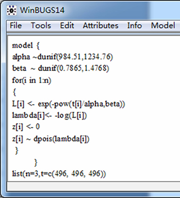
Fig. 5 BUGS model of Bayesian zero-failure problem

The operations of the checking model, loading data, compiling, and generating initial values are omitted here. The nodes (parameters) alpha and beta are set to be monitored. The length of each Markov chain is set to be 10000. The dynamic sampling traces are shown in Figs. 6 and 7.

After iteration, the first 2000 generated samples of each parameter are discarded as burn-in. The approximated probability density plots based on the remaining 8000 samples of each parameter are shown in Figs. 8 and 9.

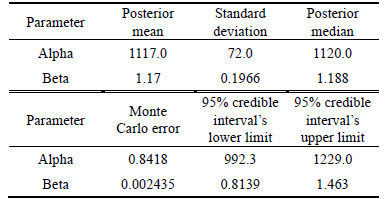
The posterior statistics obtained by the remaining 8000 samples are listed in Table 2.

According to Table 2, the posterior mean of each parameter is taken as the point estimator, given that it is commonly seen in Bayesian methods. The 95% credible interval for α is [992.3, 1229.0], and that for β is [0.8139, 1.463].

The MTBF is obtained by substituting the corresponding point estimators into Eq. (19). That is, MTBF(M)=1117.0×Γ(1+1/1.17)= 1057.9 h.

Given that the MTBFs of S₍₄₎ and S₍₅₎ are 990.9 and 1139.9 h, respectively, as shown in Section 5.3, the following relations are obtained: MTBF(S₍₄₎)< MTBF(M)(5)), which is consistent with the final expert judgment that RL(S₍₄₎)< RL(M)< RL(S₍₅₎) in Section 5.2. This consistency proves that (1) the RL-MTBF assumption in Section 3.1 is reasonable, and (2) the proposed method is able to honestly and quantitatively reflect the subjective expert judgment.

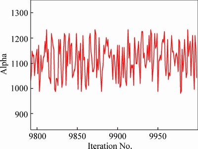
Fig. 6 Dynamic sampling trace of alpha

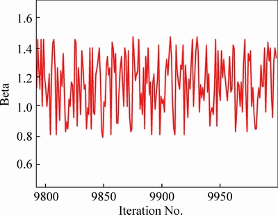
Fig. 7 Dynamic sampling trace of beta

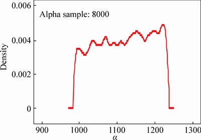
Fig. 8 Approximated PDF curve of alpha

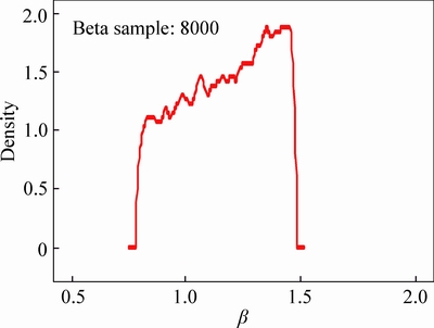
Fig. 9 Approximated PDF curve of beta

Table 2 Posterior statistics obtained by MCMC simulation in WinBUGS

However, the proposed method cannot be proven to be accurate mathematically, because the true parameter values and MTBF cannot be obtained by any methods given the zero failures. The result of MTBF can only be judged from an engineering perspective. For M, experts believe that MTBF(M)=1057.9 h is consistent with engineering realities.

6 Conclusions

1) The form of zero-failure data for multiple NCMTs and the corresponding Bayesian model are proposed.

2) An expert-judgment process is proposed to build the prior distributions of the Weibull parameters, which combines expert judgment with multi-source prior information. The Bayesian theorem combines the prior distributions with the data.

3) An MCMC algorithm is developed and run in WinBUGS, which solves high-dimensional integration, simulates the posterior distributions of the Weibull parameters, and obtains the corresponding parameter estimators. The presented BUGS model and the programming tricks provide researchers useful tools.

4) Facing zero failures in reality, a classical method, MLE, is applied to the likelihood function, given by Eq. (2). However, the results show that the solution to β is zero, which has no meaning from an engineering perspective. LSE also cannot solve the zero-failure problem.

5) From the perspective of pure statistics, the lack of failure data makes common statistics, such as the variance or length of confidence interval, meaningless to assess the proposed method. Thus, the zero-failure problem of multiple NCMTs is not a purely statistical problem, but an engineering problem. The only criterion to assess the proposed method is whether or not its results reflect the realities.

6) Although the zero-failure result in a reliability test is not expected, when it occurs, the proposed reliability modeling and assessment method aimed at zero failures of multiple NCMTs is advocated. Finally, when drawing conclusions from this method, users should state that the results are not purely mathematical values, but quantified results based on the comprehensive considerations of expert judgment, multi- source prior information, and zero-failure data.

References

[1] GUO Jun-feng, RUI Zhi-yuan, FENG Rui-cheng, WEI Xing-chun. Imperfect preventive maintenance for numerical control machine tools with log-linear virtual age process [J]. Journal of Central South University, 2014, 12(21): 4497-4502.

[2] YANG Zhao-jun, CHEN Chuan-hai, CHEN Fei, LI Guo-fa. Progress in the research of reliability technology of machine tools [J]. Journal of Mechanical Engineering, 2013, 49(20): 130-139. (in Chinese)

[3] KELLER A Z, KAMATH A R R, PERERA U D. Reliability analysis of CNC machine tools [J]. Reliability Engineering, 1982, 3(6): 449-473.

[4] JIA Ya-zhou, WANG Mo-lin, JIA Zhi-xin. Probability distribution of machining center failures [J]. Reliability Engineering and System Safety, 1995, 50(1): 121-125.

[5] YANG Zhao-jun, CHEN Chuan-hai, CHEN Fei, HAO Qing-bo, Xu Bin-bin. Reliability analysis of machining center based on the field data [J]. Eksploatacja i , 2013, 15(2): 147-155.

[6] MARTZ H F, WALLER R A. A Bayesian zero-failure (BAZE) reliability demonstration testing procedure [J]. Journal of Quality Technology, 1979, 11(3): 128-138.

[7] COOLEN F P A, COOLEN-SCHRIJNER P, RAHROUH M. Bayesian reliability demonstration for failure-free periods [J]. Reliability Engineering and System Safety, 2005, 88(1): 81-91.

[8] COOLEN F P A, COOLEN-SCHRIJNER P. On zero-failure testing for Bayesian high-reliability demonstration [J]. Proceedings of the Institution of Mechanical Engineers, Part O: Journal of Risk and Reliability, 2006, 220(1): 35-44.

[9] FAN Tsai-hung, CHANG Chia-chen. A Bayesian zero-failure reliability demonstration test of high quality electro-explosive devices [J]. Quality and Reliability Engineering International, 2009, 25(8): 913-920.

[10] YANG Guang-bin. Reliability demonstration through degradation bogey testing [J]. Reliability, IEEE Transactions on, 2009, 58(4): 604-610.

[11] MAO Shi-song, XIA Jian-feng. The hierarchical Bayesian analysis of the zero-failure data [J]. Applied Mathematics—A Journal of Chinese Universities, 1992, 7(3): 411-421.

[12] HAN Ming, DING Yuan-yao. Synthesized expected Bayesian method of parametric estimate [J]. Journal of Systems Science and Systems Engineering, 2004, 13(1): 98-111.

[13] JIANG Ping, XING Yun-yan, JIA Xiang, GUO Bo. Weibull failure probability estimation based on zero-failure data [J]. Mathematical Problems in Engineering, 2015, 2015(1): 1-8.

[14] JIANG Ping, LIM J H, ZUO Ming-jian, GUO Bo. Reliability estimation in a Weibull lifetime distribution with zero-failure field data [J]. Quality and Reliability Engineering International, 2010, 26(7): 691-701.

[15] MILLER K W, MORELL L J, NOONAN R E, PARK S K, NICOL D M, MURRILL B W, VOAS J M. Estimating the probability of failure when testing reveals no failures [J]. Software Engineering, IEEE Transactions on, 1992, 18(1): 33-43.

[16] XU Tian-qun, CHEN Yue-peng. Two-sided M-Bayesian credible limits of reliability parameters in the case of zero-failure data for exponential distribution [J]. Applied Mathematical Modelling, 2014, 38(9): 2586-2600.

[17] GUO Huai-rui, HONECKER S, METTAS A, OGDEN D. Reliability estimation for one-shot systems with zero component test failures [C]// Reliability and Maintainability Symposium (RAMS), Proceedings-Annual. San Jose: IEEE, 2010: 1-7.

[18] WALLS L, QUIGLEY J. Building prior distributions to support Bayesian reliability growth modelling using expert judgement [J]. Reliability Engineering and System Safety, 2001, 74(2): 117-128.

[19] MEYER M A, BOOKER J M. Eliciting and analyzing expert judgment: A practical guide [M]. Philadelphia: SIAM, 2001: 18-19.

[20] KAMINSKIY M P, KRIVTSOV V V. A simple procedure for Bayesian estimation of the Weibull distribution [J]. Reliability, IEEE Transactions on, 2005, 54(4): 612-616.

[21] BERGER J O. Statistical decision theory and Bayesian analysis [M]. Berlin: Springer Science & Business Media, 2013: 83-84.

[22] HAMADA M S, WILSON A, REESE C S, MARTZ H. Bayesian reliability [M]. Berlin: Springer Science & Business Media, 2008: 51-52.

[23] NEAL R M. Slice sampling [J]. Annals of Statistics, 2003, 31(3): 705-767.

[24] WANG Xiao-lin, GUO Bo, CHENG Zhi-jun, JIANG Ping. Residual life estimation based on bivariate Wiener degradation process with measurement errors [J]. Journal of Central South University, 2013, 20(7): 1844-1851.

[25] LUNN D, JACKSON C, BEST N, THOMAS A, SPIEGELHALTER D. The BUGS book: A practical introduction to Bayesian analysis [M]. Boca Raton: CRC press, 2012: 204-205.

[26] MURTHY D N P, XIE Min, JIANG Ren-yan. Weibull models [M]. Hoboken: John Wiley & Sons, 2004: 54-55.

(Edited by YANG Bing)

Foundation item: Project(2014ZX04014-011) supported by State Key Science & Technology Program of China; Project([2016]414) supported by the 13th Five-year Program of Education Department of Jilin Province, China

Received date: 2015-08-08; Accepted date: 2015-10-26

Corresponding author: LI Guo-fa, Professor, PhD; Tel: +86-13843069140; E-mail: ligf@jlu.edu.cn