J. Cent. South Univ. Technol. (2011) 18: 429-437

DOI: 10.1007/s11771-011-0714-6

Nonlinear optimal control for robotic yoyo playing

YUAN De-hu(袁德虎)^{1, 2}, JIN Hui-liang(金惠良)¹, MENG Guo-xiang(孟国香)¹

1. School of Mechanical Engineering, Shanghai Jiao Tong University, Shanghai 200240, China;

2. Research and Development Center, Shanghai Aerospace Control Engineering Institute, Shanghai 200233, China

? Central South University Press and Springer-Verlag Berlin Heidelberg 2011

Abstract: A general approach for controlling of periodical dynamic systems was presented by taking robotic yoyo as an example. The height of the robot arm when the yoyo arrives at the bottom was chosen as virtual control. The initial amplitude of yoyo could be mapped to the desired final amplitude by adjusting the virtual control. First, the yoyo motion was formulated into a nonlinear optimal control problem which contained the virtual control. The reference trajectory of robot could be obtained by solving the optimal problem with analytic method or more general numerical approach. Then, both PI and deadbeat control methods were used to control the yoyo system. The simulation results show that the analytic solution of the reference trajectory is identical to the numerical solution, which mutually validates the correctness of the two solution methods. In simulation, the initial amplitude of yoyo is set to be 0.22 m which is 10% higher than the desired final amplitude of 0.2 m. It can be seen that the amplitude achieves the desired value asymptotically in about five periods when using PI control, while it needs only one period with deadbeat control. The reference trajectory of robot is generated by optimizing a certain performance index; therefore, it is globally optimal. This is essentially different from those traditional control methods, in which the reference trajectories are empirically imposed on robot. What’s more, by choosing the height of the robot arm when the yoyo arrives at the bottom as the virtual control, the motion of the robot arm may not be out of its stroke limitation. The proposed approach may also be used in the control of other similar periodical dynamic systems.

Key words: robotic yoyo; return map; reference trajectory; optimal control

1 Introduction

Yoyo playing represents a class of periodical unstable dynamic manipulation which involves cyclic exchange of kinetic energy and potential energy under gravitation. Other similar tasks include hopping [1-3], brachiating [4-7] and juggling [8-10] etc. Some researchers have studied robotic yoyo playing [11-15]. The control in Ref.[11] is based on a nominal reference trajectory for the robot. A main disadvantage of this method is that only the amplitude of the reference trajectory can be adjusted, while its period is fixed. Recently, JIN and ZACKSENHOUSE [12-13] proposed a model-based approach and a neural-based one. The former relies heavily on the mathematical model of the specific task, while the latter closely depends on the specific behavior—phase locking. Essentially, all the control ideas are heuristic to some extent and rely on the distinctive dynamics of the specific tasks, which is far from a well-developed general approach to control such applications.

Recently, JIN et al [14] presented a unified method to nominal control generation for yoyo playing, and gave the analytic solution. The approach is based on choosing the velocity of yoyo at the bottom as the virtual control, and assuming that the robot has in?nite ability and can follow precisely any smooth reference trajectory. The major drawback of this method is that it neglects the actual stroke limitation of the arm of robot. For example, the stroke is only 0.2 m for the Z axle of the cartesian robot which has been successfully used for yoyo playing based on the model control in our laboratory.

In this work, the height (h_b) of the robot arm when the yoyo is at the bottom was chosen as the virtual control, that is, the initial amplitude of yoyo could be mapped into the desired final amplitude by controlling h_b. This guarantees that the motion of the robot arm may not be out of its stroke limitation. For the optimal control problem, not only was the analytic solution given, but also a more general numerical-solution method was presented. The reference trajectory of robot was generated by optimizing a certain performance index. This is essentially different from those methods in Refs.[11-13], in which the reference trajectories are all empirically imposed. Therefore, the approach proposed in this work is of much generality, which may also be used in the control of other similar periodical dynamic systems.

2 Yoyo model

The simple one-degree of freedom (DOF) model established in Ref.[15] is used here. The model adequately describes the total energy loss of yoyo and has been successfully testified in Refs.[12-13] for analysis, simulation, and real-time control.

As described in Ref.[15], the one-DOF model is derived from a more detailed two-DOF model by capturing the dynamics at the bottom with an equivalent restitution effect e_eq. Let the mass and the inertia of the yoyo be m and I, respectively, the radii of the axle and the disk of the yoyo be r and R, respectively, the rotational angle be θ, the total length of the string be L, and the height of the yoyo center and the robot be y and h, respectively (see Fig.1). When the yoyo is rolling down or up the string, its dynamics is governed by

                                   (1)

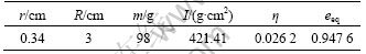
where η=mr²/(I+mr²) (Table 1 lists the values of the parameters).

When the yoyo hits the bottom at a time t_b, its dynamics may be captured by a restitution effect:

       (2)

where e_eq=1-2η, is the equivalent coefficient of restitution, provided that η is not larger than 1/2 and the superscripts “-”and “+” stand for the moment immediately before and after the restitution effect, respectively.

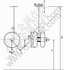
Fig.1 Schematic illustration of yoyo

Table 1 Parameters of yoyo

In the configuration, the origin of θ is selected to be the state such that the string is fully unwound and Eq.(1) is used for both the downward and the upward motions. It is understood that the angular velocity  is negative when the yoyo is unwinding, and positive when it is winding up the string. When the yoyo hits the bottom,  changes its sign, as given in Eq.(2), even though the direction of rotation does not change.

From the perspective of control, θ and  are the state variables, y is the output signal to be measured, and h is the input to be designed.

According to the yoyo model, the optimal control problem can be expressed as

                                (3)

where the state is

                        (4)

and the control is

                                                         (5)

3 Division of motion into periods

First, the motion of the yoyo is divided into periods. While this division is not unique, there are two important guidelines to follow.

1) Smoothness: for a smooth transition between two consecutive periods, the periods should start when the motion of both the robot and the object is smooth.

2) Minimal number of discontinuities: it is possible that each period may have more than one discontinuous point. In order to avoid unnecessary parameters appearing in the return map, the division should be selected to minimize the number of discontinuous points in each period—just enough to perform a desired manipulation. For example, the period of one-bat control law (1BCL) in Ref.[16] has one discontinuous point, which is just enough, and that of 2BCL has two such points, which is more than just enough.

Accordingly, the yoyo movement is divided into periods which start at the apex points of the yoyo, when the robot is usually at its bottom position and almost stationary. Each period has only one discontinuous point. When the yoyo is at the bottom at time t_b, as illustrated in Fig.2, its angular velocity  is not continuous, and its angular position is therefore not smooth. This point divides each period of the yoyo into two phases, one down and one up. The motion can be described by a simplified dynamic model with an impulsive effect at the bottom (see Eq.(2)).

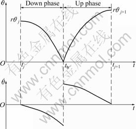
Fig.2 Yoyo motion period divided into two phases

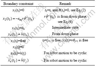
The boundary constraints for the two phases are listed in Table 2 and Table 3.

Table 2 Boundary constraints of down phase

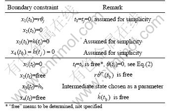
Table 3 Boundary constraints of up phase

4 Optimal programming

4.1 Basic problem

Basic dynamic programming problem of nonlinear optimal control is to find a control u(t) and the possibly free final time t_f, which can minimize the performance index:

             (6)

A vector of initial, final and trajectory constraints must be satisfied:

                (7)

And the system  is also a trajectory constraint.

The performance index is chosen as

                                             (8)

which represents the effort of the robot in each phase. For simplicity, let

                                      (9)

Following a standard routine (see Refs.[17-18] for details), the optimal control problem is solved phase by phase.

Introduce a Lagrange multiplier and construct a Hamiltonian:

              (10)

The multiplier (or co-state) equation is

                                (11)

The control equation

                  (12)

Solving (11) and (12) yields

                                            (13)

where C₁, …, C₄ are constants to be determined, and

                              (14)

Substituting Eq.(14) into Eq.(3) and solving the system equation gives

(15)

For simplicity, in the following derivation of the coefficients, it is assumed that t₀=0 in the two phases.

4.2 Down phase

With the four initial constraints listed in Table 2, the coefficients, B₁, …, B₄, can be easily determined as

                                         (16)

With the two terminal constraints which are not marked “free”, it gives

  (17)

The two “free” terminal constraints imply that

                           (18)

Letting H=0 along the optimal trajectory and combining with Eq.(10) and Eqs.(13)-(18), the coefficients, C₁, …, C₄, and t_f are finally solved as

                    (19)

                                      (20)

Substituting Eq.(16) and Eq.(19) into Eq.(14) and Eq.(15), finally the optimal solution in down phase is obtained as

                                   (21)

and the optimal control is

                                            (22)

where

                           (23)

With Eqs.(20), (21) and (23), the velocity of yoyo and the arm of robot when the yoyo hits the bottom can be respectively calculated as

             (24)

and

                           (25)

They will be used as the initial constraints in the following up phase.

4.3 Up phase

In the same way, with the initial constraints listed in Table 3, the coefficients, B₁, …, B₄, are determined as

                                             (26)

where  and  are given in Eq.(24) and Eq.(25), respectively.

For simplicity of derivation, let

                                           (27)

With Eqs.(15), (26), (27) and three terminal constraints that are not marked “free”, the following equations will be obtained:

       (28)

Substituting Eqs.(24) and (25) into Eq.(28) and solving the equations yields

     (29)

                      (30)

Therefore, the optimal solution in up phase is

           (31)

and the optimal control is

                                                 (32)

According to the above deduction, for the optimal control problem, two propositions are given below.

Proposition 1 For the performance index (Eq.(6) and Eq.(8)), the yoyo model (Eq.(3)), and the motion period shown in Fig. 2 with the boundary constraints given in Table 2 and Table 3, the optimal nominal control is

           (33)

where the coefficients A, C, C_a, C_b and the times t_b, t_j+1 are all functions of rθ_j and h_b.

Proof Shifting t₀=0 back to t₀=t_b in Eqs.(22) and (32), it yields the upper and lower half of Eq.(33), respectively.

Proposition 2 The optimal nominal control (Eq.(33)) results in the following return map:

  (34)

Proof Substituting Eq.(30) into the first equation of Eq.(31), the return map can be obtained as Eq.(34).

With the solution (Eq.(21) and Eq.(31)), the state curve can be obtained, as shown in Fig.3. The initial amplitude of the yoyo is 0.2 m. The solid curve is obtained deliberately with the return map (Eq.(34)), so that the final amplitude rθ_j+1 retains the initial value. The figure also shows that rθ_j+1 increases with the value of h_b near the equilibrium point.

5 Control scheme and simulation

With return map (Eq.(34)), it is not difficult to get the fixed point:

                                                  (35a)

or

                                         (35b)

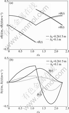
Fig.3 State curves of one period with analytic solution:      (a) Curves of rθ(t) and  (b) Curves of h(t) and

Let rθ*=0.2 m, then h_b can be calculated as

m

It obviously exceeds the stroke of the arm of an ordinary robot, therefore Eq.(35a) is of no physical significance and should be abandoned.

It can be demonstrated that the fixed point (Eq.(35b)) is unstable; therefore, feedback control should be utilized to stabilize the whole system. To this end, the return map (Eq.(34)) can be viewed as a discrete-time system with the intermediate state h_b as a virtual control, i.e.

                                (36)

Thus, a discrete control law may be used:

                                          (37)

where rθ_d represents the desired amplitude of the yoyo.

Fig.4 shows the block diagram for the control of yoyo. The final amplitude rθ_j of the former period becomes the initial amplitude of the current period through the period-wise feedback. In real-time control, the initial amplitude of yoyo in each period is measured by a camera. The nominal control (Eq.(33)) may be adjusted by the coefficients A, C, C_a, C_b which are parameterized by rθ_j and h_b. And h_b is also adjusted through the discrete control. The above process may be repeated period by period in order that the overall system may be stable.

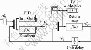
Fig.4 Block diagram for control of yoyo

Several simple discrete-time control laws, such as PID and deadbeat control, can be used for the scalar system (Eq.(34)). Here, a PI control is given by

           (38a)

where

                                   (38b)

which can be obtained by replacing rθ^* with rθ_d in Eq.(35b).

Solving the return map (Eq.(34)) for h_b and replacing rθ_j+1 with rθ_d yields the deadbeat control law as

   (39a)

or

  (39b)

where

                 (39c)

Similarly, Eq.(39b) is of no physical significance and should be given up.

Fig.5 shows the simulation response curve under PI control (Eq.(38)) with proportional gain K_p=3 and integral gain K_i=0.5. The initial amplitude, rθ₀, is set to be 0.22 m which is 10% higher than the desired value rθ_d=0.2 m. It can be seen that the amplitude rθ_j achieves the desired value gradually in about 5 periods. Fig.6 shows the response curves with deadbeat control (Eq.(39)), and the initial amplitude is also set to be  0.22 m. This shows that rθ_j achieves the desired value immediately in only one period.

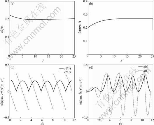
Fig.5 Response curves for PI control: (a) Response of rθ_j; (b) Response of  (c) Curves of rθ(t) and  (d) Curves of h(t) and

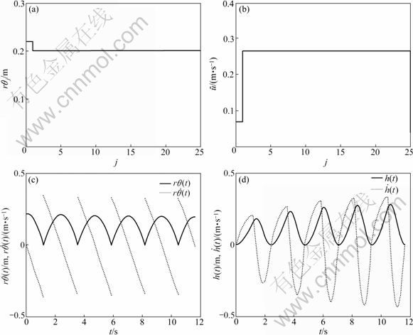
Fig.6 Response curves for deadbeat control: (a) Response of rθ_j; (b) Response of  (c) Curves of rθ(t) and  (d) Curves of h(t) and

6 Numerical solution

While the optimal control problem for the yoyo example is solved analytically, it is generally not guaranteed that any nonlinear optimal control problem can be solved in this way. The solution of general optimal control problems usually requires numerical methods.

For the optimal programming problem, the numerical solving process proposed in this work is based on the inversion-based optimization technique [19-20], which utilizes the NTG (Nonlinear Trajectory Generation) software package developed at Caltech. The NTG algorithm is a gradient descent optimization method that combines three technologies: B-splines, output space collocation and nonlinear optimization tools [21]. NTG is based on two other FORTRAN packages: NPSOL and PGS. NPSOL (Nonlinear Programming of Systems Optimization Laboratory) is a numerical optimization library developed by Stanford University, and it uses sequential quadratic programming to solve nonlinear optimization problems. PGS is the Practical Guide to Splines companion software [22].

The boundary constraints listed in Table 2 and Table 3, the nonlinear trajectory constraint (Eq.(3)), and the unintegrated cost function (Eq.(8)) etc. are formulated in C language in the NTG program. The time t and two state variables, rθ and h, are chosen as the output variables. A second order B-spline with one knot interval and C¹ continuity across the knot points is chosen to parameterize the first output. The fifth order B-splines with one knot interval again but C³ continuity are chosen to parameterize the other two outputs. Totally, twelve coefficients are to be solved in each phase. For each coefficient, an initial value of 1.0 is assigned arbitrarily.

A modified version of the routine ZBRENT [23] was used for root finding. The above NTG program for one period was called iteratively by the routine until a desired  such that rθ_j+1=rθ_j was found. The interval chosen for the routine was [0.01, 0.99] and the termination tolerance was e_tol=10^-4. The initial amplitude and the desired amplitude were the same (0.2 m). The number of breakpoints was n_bps=11. Finally, it used 3 periods to find the desired 0.261 5, corresponding to which the B-spline coefficients of down phase and up phase were numerically solved as

c_down=[0  1.143 3  0.2  0.2  0.116 1  0.009  0  0 

0  0.063 5  0.162 9  0.261 4]

and

c_up=[0  1.143 3  0  0.093 1  0.162  0.2  0.261 4

0.25  0.197 9  0]

Multiplying these coefficients with corresponding collocation matrices yields the matrices for the state variables rθ,  h and  With these state matrices, the simulated state curves can be obtained, as shown in Fig.7. It can be seen that the curves are identical with the solid curves in Fig.3, in which the initial amplitudes are all the same to the final amplitudes. And this mutually demonstrates the correctness of the analytic and numerical methods.

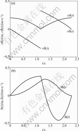
Fig.7 State curves of one period with numerical solution:    (a) Curves of rθ(t) and  (b) Curves of h(t) and

7 Conclusions

1) Based on the nonlinear optimal control and using the period-wise feedback and period-wise trajectory- planning, a unified method for controlling cyclic dynamics is presented. In the context of yoyo playing, the approach includes three main steps. First, divide the motion of the yoyo into periods and determining the boundary conditions. Second, look for an appropriate intermediate state (e.g. h_b) of the yoyo or robot within a period as the virtual control. Finally, design an optimal control problem with appropriate initial, final, and trajectory constraints that incorporate the intermediate state of the yoyo or robot.

2) By solving the optimization problems phase by phase in each period, a reference trajectory for the robot is obtained analytically or numerically, and the associated return map is evaluated. With the return map obtained, standard analysis and design methods for discrete-time systems can be applied to control the dynamic system in real time.

References

[1] NELSON N, HANAK T, LOEWKE K, MILLER D N. Modeling and implementation of McKibben actuators for a hopping robot [C]// Proceedings of the 12th International Conference on Advanced Robotics. Seattle: IEEE, 2005: 833-840.

[2] CHEROUVIM N, PAPADOPOULOS E. Single actuator control analysis of a planar 3DOF hopping robot [C]// Robotics: Science and Systems I. Cambridge: MIT Press, 2005: 145-152.

[3] CHEROUVIM N, PAPADOPOULOS E. Energy saving passive-dynamic gait for a one-legged hopping robot [J]. Robotica, 2006, 24: 491-498.

[4] OLIVEIRA V M, LAGES W F. Comparison between two actuation schemes for underactuated brachiation robots [C]// Proceedings of the International Conference on Advanced Intelligent Mechatronics. Zurich: IEEE/ASME, 2007: 1-6.

[5] GOMES M W, RUINA A L. A five-link 2D brachiating ape model with life-like zero-energy-cost motions [J]. Journal of Theoretical Biology, 2005, 237: 265-278.

[6] OLIVEIRA V M, LAGES W F. MPC applied to motion control of an underactuated brachiation robot [C]// Proceedings of the Conference on Emerging Technologies & Factory Automation. Prague: IEEE, 2006: 985-988.

[7] OLIVEIRA V M, LAGES W F. Linear predictive control of a brachiation robot [C]// Proceedings of the Conference on Electrical and Computer Engineering. Ottawa: IEEE, 2006: 1518-1521.

[8] HIRAI H, MIYAZAKI F. Dynamic coordination between robots: self-organized timing selection in a juggling-like ball-passing task [J]. IEEE Transactions on Systems, Man, and Cybernetics, 2006, 36(4): 738-754.

[9] NAKASHIMA A, SUGIYAMA Y, HAYAKAWA Y. Paddle juggling of one ball by robot manipulator with visual servo [C]// Proceedings of the 9th International Conference on Control, Automation, Robotics and Vision. Singapore: IEEE, 2006: 1-6.

[10] BROGLIATOA B, MABROUKB M, RIOC A Z. On the controllability of linear juggling mechanical systems [J]. Systems & Control Letters, 2006, 55: 350-367.

[11] HASHIMOTO K, NORITSUGU T. Modeling and control of robotic yoyo with visual feedback [C]// Proceedings of the International Conference on Robotics and Automation. Minneapolis: IEEE, 1996: 2650-2655.

[12] JIN H L, ZACKSENHOUSE M. Robotic yoyo playing with visual feedback [J]. IEEE Transactions on Robotics, 2004, 20(4): 736-744.

[13] JIN H L, ZACKSENHOUSE M. Oscillator-based yoyo control: implementation and comparison with model-based control [C]// Proceedings of the 12th International Conference on Advanced Robotics. Seattle: IEEE. 2005: 153-158.

[14] JIN H L, YE Q, ZACKSENHOUSE M. Return maps, parameterization, and cycle-wise planning of yo-yo playing [J]. IEEE Transactions on Robotics, 2009, 25(2): 438-445.

[15] JIN H L, ZACKSENHOUSE M. Yoyo dynamics: sequence of collisions captured by a restitution effect [J]. Journal of Dynamic Systems, Measurement and Control, 2002, 124(3): 390-397.

[16] LYNCH K M, BLACK C K. Recurrence, controllability, and stabilization of juggling [J]. IEEE Transactions on Robotics and Automation, 2001, 17(2): 109-123.

[17] BRYSON A E, HO Y C. Applied optimal control: optimization, estimation, and control [M]. Washington: Hemisphere, 1975.

[18] NAIDU D S. Optimal control systems [M]. Cambridge: Cambridge University Press, 2003.

[19] MILAM M B, MUSHAMBI K, MURRAY R M. A new computational approach to real-time trajectory generation for constrained mechanical systems [C]// Proceedings of the Conference on Decision and Control. Sydney: IEEE, 2000: 845-851.

[20] PETIT N, MILAM M B, MURRAY R M. Inversion based constrained trajectory optimization [C]// Proceedings of the 5th Symposium on Nonlinear Control Systems. Petersburg: IFAC, 2001: 1211-1216.

[21] MISOVEC K, INANC T, WOHLETZ J, MURRAY R M. Low-observable nonlinear trajectory generation for unmanned air vehicles [C]// Proceedings of the 42nd Conference on Decision and Control. Hawaii: IEEE, 2003: 3103-3110.

[22] DE BOOR C. A practical guide to splines [M]. New York: Spring- Verlag, 1978.

[23] PRESS W H. Numerical recipes in C++, 3rd edition [M]. New York: Cambridge University Press, 2007.

(Edited by YANG Bing)

Foundation item: Project(50475025) supported by the National Natural Science Foundation of China

Received date: 2009-08-24; Accepted date: 2009-12-17

Corresponding author: YUAN De-hu, PhD; Tel: +86-13564325001; E-mail: dehuyuan@gmail.com