
J. Cent. South Univ. (2016) 23: 240-248
DOI: 10.1007/s11771-016-3067-3

Oil–water two-phase flow pattern analysis with ERT based measurement and multivariate maximum Lyapunov exponent
TAN Chao(谭超), WANG Na-na(王娜娜), DONG Feng(董峰)
Tianjin Key Laboratory of Process Measurement and Control
(School of Electrical Engineering and Automation, Tianjin University), Tianjin 300072, China
 Central South University Press and Springer-Verlag Berlin Heidelberg 2016
Abstract:
Oil–water two-phase flow patterns in a horizontal pipe are analyzed with a 16-electrode electrical resistance tomography (ERT) system. The measurement data of the ERT are treated as a multivariate time-series, thus the information extracted from each electrode represents the local phase distribution and fraction change at that location. The multivariate maximum Lyapunov exponent (MMLE) is extracted from the 16-dimension time-series to demonstrate the change of flow pattern versus the superficial velocity ratio of oil to water. The correlation dimension of the multivariate time-series is further introduced to jointly characterize and finally separate the flow patterns with MMLE. The change of flow patterns with superficial oil velocity at different water superficial velocities is studied with MMLE and correlation dimension, respectively, and the flow pattern transition can also be characterized with these two features. The proposed MMLE and correlation dimension map could effectively separate the flow patterns, thus is an effective tool for flow pattern identification and transition analysis.
Key words:
1 Introduction
Oil–water two-phase flow is frequently seen in petroleum industries and other similar production lines. The flow patterns of oil–water flow are important to understand the flow rheology and mechanisms [1]. The oil–water flow is complex in structures since the interfaces between oil and water are not usually explicit, and the flow system demonstrates a time-variant and complex phase distribution when changing flow conditions [2].
Many sensing techniques have been used to analyze the flow patterns of oil–water two-phase flow, including the particle image velocimetry (PIV) and particle tracking velocimetry (PTV) [3], impedance probes [4] and image analysis with a high speed camera [5]. Among these methods, the impedance methods have the advantages of low cost, non-intrusive and easy installation, thus can be used not only in the lab scale, but also in plant scale analysis.
In most of the published literatures, flow patterns are characterized by using a single sensor and univariate time-series analysis methods. By analyzing this univariate measurement history, the hidden mechanism of flow patterns can be uncovered. However, these methods are limited to the averaged or single-pointed local information regarding the flow process, so the information extracted by using these methods does not contain a variety of the flow structural information important to reflect the structural change of flow patterns. Therefore, the multiple sensors are needed to deliver more comprehensive information for two-phase flow analysis.
As a multi-electrode impedance method, the electrical tomography has gained attentions in two-phase flow analysis in the past few decades. According to the properties of the fluid that an electrical tomography is sensitive to, the electrical tomography is grouped into electrical resistance tomography (ERT), electrical capacitance tomography (ECT) and electromagnetic tomography (EMT). ERT and ECT are frequently used in oil–water, gas–liquid two-phase flow analysis due to their fast response to flow conditions. ERT operates properly when the continuous phase is electrically conductive, while ECT operates properly when the conductivity of the continuous phase is low [6]. Thus, for the oil–water two-phase flow analysis, ERT works well in the water continuous flow and ECT in the oil continuous flow. For example, an ERT was used in the flow pattern identification with a single vector [7], however, the flow pattern analysis is hard to uncover by using the single vector based time-series.
By using tomography methods, the multiple electrodes deliver the multivariate data consisting of local information of phase distribution and fraction. These multivariate data provide simultaneous response to the flow patterns from different locations [8]. Synthesizing the local information provides a comprehensive characterization of flow structures. Under this frame work, many methods of multivariate time- series analysis can be adopted, such as the multivariate multiscale entropy analysis for the gas–water two-phase flow pattern characterizations [9]. The oil–water two- phase flow is a complex dynamic system that shows the chaotic behavior over time; therefore, the chaotic analysis method can also be applied. The maximum Lyapunov exponent (MLE) [10], usually extracted from a univariate time-series, is an index characterizing the complexity of a dynamic system. Considering the limitation of the univariate analysis discussed above, the MLE needs to move to the multivariate analysis to include more information for system dynamic analysis, such as the multivariate MLE (MMLE) [11]. If treated as a multivariate time-series, the high-dimensional measurement of an ERT provides an MMLE to characterize the flow structure. Correlation dimension is another index to characterize the self-similarity of a chaotic system, which can also be used for flow analysis.
In the present work, the measurement of ERT is used to analyze the oil–water two-phase flow patterns in a horizontal pipe. Typical flow patterns were observed in a set of dynamic experiments in a multiphase flow facility. The MMLE along with the correlation dimension [12–13] was extracted from the 16-electrode ERT measurement to characterize the flow patterns. These two features can jointly characterize and separate the flow patterns on a MMLE to correlation dimension map.
2 ERT and MMLE
2.1 Electrical resistance tomography
The operating principle of an electrical resistance tomography (ERT) is that the conductivity varies between fluids. For a two-phase flow system, usually one-phase fluid has a higher conductivity than other phases. Thus, by injecting a known/constant amplitude electric current into the two-phase mixture, the resulted voltage will change with the resistance of the mixture. This mixture resistance is directly related to the phase distribution and phase fraction within the cross-section. In order to reconstruct the cross-sectional image, more measurement is needed to achieve a high resolution of the phase distribution. By doing this, an ERT evenly implements a number of electrodes on the periphery of one cross section of the target vessel. Then, by injecting the stimulating electric current through a pair of electrodes and measuring the voltages between each pair of the neighboring electrodes, the information regarding phase distribution at each excitation is obtained. Repeating this process till all the electrodes have been stimulated and all the voltages are collected, a set of data is acquired which is usually called a frame. This operating principle is named the adjacent mode, as shown in Fig. 1.
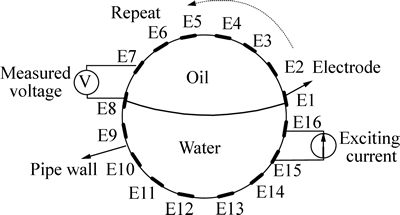
Fig. 1 Operating principle of ERT
The ERT system used in the present work is a 16-electrode parallel data acquisition ERT system. It collects 150 frames data (208 measurement in each frame) per second, thus providing a 208-dimensional time-series data after a length of time in dynamic experiments [14].
2.2 Multivariate maximum Lyapunov exponent
Before calculating the maximum Lyapunov exponent, the multivariate time-series needs to be reconstructed in the phase space [15]. The selection of the embedding dimension and delay time has direct effect on the calculation of the maximum Lyapunov exponent.
Let  (i=1, 2, …, M) be the observation time-series of M variables, where N is the length of the time-series. Apply the C-C algorithm [16–17] to each time-series, so the optimized embedding dimension and time delay can be obtained through the following reconstructed phase space for the multivariate time-series:


 (1)
(1)
where n=N0, N0+1, …, N, N0= and mi and τi are the embedding dimension and time delay of the ith time-series.
By changing the time-series from time domain into the frequency domain with the fast Fourier transform (FFT), the average period of the chaotic time-series, P, can be obtained by calculating the frequency information in the frequency domain.
After FFT, time series {x(t), t=1, 2, …, N} becomes
 (2)
(2)
The frequency during the above transform is
 (3)
(3)
Weight-average the power to obtain the average period:
 (4)
(4)
The multivariate maximum Lyapunov exponent can be calculated with the small set method [18]. After reconstructing the phase space of the multivariate time series, find the nearest point  of each point Xn. Make sure these two points are in different tracks by maintaining a certain separation dn(0) between them.
Assume that dn(0) is the separation between the nearest point and point Xn:
 (5)
(5)
where P is the average period.
Calculate the distance of the nearest point of Xn after the ith evolution by assuming that the nearest point of Xn diverges in the rate of maximum Lyapunov exponent:
 (6)
(6)
Assume that point Xn and its nearest point separate in an exponent distance:
 (7)
(7)
where Cn is the initial separation, and λ is the MLE coefficient.
The logarithmic form of Eq. (7) is
 (8)
(8)
where i=1, 2, …, min(N–N0+1–n, N–N0+1–
Calculate the averaged y(i) to all the lndn(i):
 (9)
(9)
where k is the number of non-zero dn(i). The slope of this curve after least square fitting is the maximum Lyapunov exponent.
2.3 Correlation dimension
Another important index to characterize a dynamic system is the correlation dimension. It reflects the self- similarity and randomness of the system. For an M-variate time-series, the phase space is firstly reconstructed with C-C algorithm, and then the correlation integral is defined as
 (10)
(10)
where Xi and Xj are the two points in the phase space reconstruction, and H(x) is the Heaviside function defined as
 (11)
(11)
Therefore, the correlation dimension is calculated with
 (12)
(12)
The correlation dimension D is the slope of curve lnC(r)–lnr meeting the requirement of 1/2Dstd<>std, where Dstd is the standard deviation of time-series.
3 Experiments
3.1 Experiment facility
The oil–water two-phase flow experiments were conducted on a multiphase flow facility in Tianjin University (China). The structure of the testing rig is shown in Fig. 2. The horizontal pipe is made of stainless steal with 50 mm in inner diameter and 16 m in length. The ERT system introduced above was implemented at 14 m downstream from the inlet of the horizontal pipe. The mineral white oil (density of 790 kg/m3 and dynamic viscosity of 0.029 Pa·s) and tap water (density of 998 kg/m3 and dynamic viscosity of 0.001 Pa·s) were pumped into the horizontal pipe, respectively, from their own storage tank. They were mixed at the inlet and fully developed into stable flow patterns at the test section. By controlling the flow rate of each individual flow rate, oil–water two-phase flow of different phase fractions and overall flow rate was formed for the investigation of flow patterns. A digital camera recorded the flow patterns through a transparent section of the pipeline. The water holdup was from 33% to 100% where only the water continuous flow occurred, so ERT worked properly in this range. Water superficial velocity was from 0.28 m/s to 1.96 m/s, and oil superficial velocity was from 0 m/s to 1.13 m/s.
3.2 Flow patterns in experiments
Since the ERT can only operate properly when the continuous phase is water, only water continuous flow patterns were recorded, including stratified flow with mixing interface (ST&MI) flow, dispersion of oil droplets in water and water (Do/w&w) flow, dispersion of water in oil and the dispersion of oil in water (Dw/o&Do/w) flow, and oil dispersion in water (o/w) flow. The flow patterns and their corresponding flow conditions are plotted in Fig. 3 to compare with the flow pattern transition presented by TRALLERO et al [19].

Fig. 2 Test facility for oil–water two-phase flow experiment

Fig. 3 Flow patterns and conditions in experiments
The photos of these typical flow patterns are shown in Fig. 4. The ST&MI flow has two continuous layers: oil flows at the top and water at the bottom. An oil-droplets layer flows at the interface of oil and water, which is caused by the vortex at the interface. By increasing the water superficial velocity, the water phase fraction increases and the dynamic energy possessed by the high velocity water flow breaks the continuity of the oil layer, forming dispersed oil droplets flowing inside the water and a continuous water layer at the bottom. This flow condition is named Do/w&w flow. The oil dispersion layer induces more fluctuations than the oil layer in ST&MI flow. Increasing the oil velocity, both the SI&MI flow and the Do/w&w flow change into the Dw/o&Do/w flow. It has two dispersion layers of the water droplets in the oil flowing at the top, and the oil droplets in the water at the bottom. Because the oil droplets at the top start coalescing into big bubbles and finally into the continuous phase when oil phase fraction increases, the high dynamic energy of the two-phase mixture makes the oil layer entrain the water droplets flowing together, forming the water in oil dispersion layer. Meanwhile, the high velocity oil phase breaks the continuity of the water layer at the bottom, so the oil droplets disperse inside the water, forming the water dispersion layer. Since this flow pattern occurs at high superficial velocity and oil phase fraction, it will eventually change into the oil continuous flow. i.e. the phase inversion occurs [20]. At the low oil phase fraction and high overall superficial velocity of the two-phase flow, a fine dispersion of oil in water is formed, which is the o/w flow. In this flow pattern, the oil phase cannot form a continuous layer due to the turbulence of the high velocity fluid, and the dynamic energy prevails the gravity, so the oil droplets finely disperse in the water without accumulating at the top of the pipe.
4 Flow pattern analysis
4.1 Data pre-processing
The information extracted from each electrode contains the information that is directly related to the position where the stimulated electrode is installed. Therefore, each electrode is treated as a single sensor that collects the local phase fraction change information. For each frame of data, 208 measurements need to be processed to extract the local flow information. This is a large matrix if considering an interval of detecting time- series of each measurement. Therefore, this measurement matrix needs to be compressed into a one-dimensional vector:
 (13)
(13)
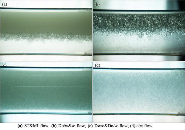
Fig. 4 Photos of oil-water two-phase flow patterns in experiments:
where Vij0 is the j (j=1, 2, …, 13) measured voltage when the i (i=1, 2, …, 16) electrode is stimulated with the pipe filled with water, and Vij is the corresponding measured voltage of two-phase flow. After pre- processing, a 16-dimensional feature time-series V is formed, and each VN,i represents the ith time-series with N measurement in time (N=1000). The 16-variate time- series of ERT consists of the local phase fraction/ distribution information at each electrode. By applying the multivariate analysis methods, a comprehensive description on the phase distribution and fluctuation both in the spatial and the time domain can be drawn.
4.2 MMLE of different flow patterns
Reconstruct the phase space with C-C algorithm to each time-series VN,i, so the embedding dimension mi and time delay τi are obtained, and the multivariate time- series Vn is reconstructed in the phase space. The MMLE is obtained through the above algorithm. In addition, since the flow patterns are also dependent on the physical parameters of the two-phase flow, the ratio of water superficial velocity to oil superficial velocity, Jw/Jo, is introduced to jointly characterize the flow patterns.
Figure 5 demonstrates that MMLE of all the four flow patterns are higher than zero, indicating the chaotic properties of the oil–water flow. The o/w flow has the highest MMLE, because it consists the most disordered fluctuations. Since the ERT measures the fluctuations around the pipe, the o/s flow provides valid measurement of all the 16 electrodes. The fluctuations at each detecting electrode are different, and the fluctuations over time also show disordered behaviors due to the high superficial water velocity and the dynamic energy it possesses, thus the o/w flow shows the highest MMLE. The Dw/o&Do/w flow and the ST&MI flow have similar MMLE that is smaller than that of the o/w flow, suggesting that the dual-dispersion and the dual- continuous flow patterns (Fig. 4) have the similar complexity. These two flow patterns show macro structures over time when flowing, causing low frequency waves at the interface. Meanwhile, both flow patterns have an oil continuous layer at the upper part of the pipe, which invalidates the measurement of the electrodes dipped into the oil layer. The decrease of valid response of the multivariate time-series also reduces the value of MMLE. The Do/w&w flow has the lowest MMLE value. Since a continuous water layer exists at the bottom of the pipe, only the oil droplets in the water phase at the upper part of the pipe provide large waves to the electrodes. Meanwhile, the size of the oil droplet in the Do/w&w flow is larger than that of the o/w flow, so the fluctuations are more severe and the complexity reduces accordingly.

Fig. 5 MMLE value with different flow patterns
To further understand the flow pattern transitions with MMLE, the MMLE is plotted against the ratio of oil superficial velocity to water superficial velocity, Jo/Jw. Figure 6(a) shows the MMLE change with Jo/Jw when water superficial velocity is Jw=0.29 m/s. MMLE drops with the increase of oil superficial velocity, because the higher oil phase fraction creates more continuous flow layer and the flow structure becomes more ordered. When Jw=0.56 m/s (Fig. 6(b)), the ST&MI flow transits to Dw/o&Do/w flow when increasing the oil fraction. The MMLE drops with increasing oil superficial velocity, indicating that the decreasing of disorder only occurs in the same flow pattern. When the flow pattern transition occurs, the MMLE starts to increase, suggesting that the disorder of the flow structure alters at pattern transition. The MMLE then drops with oil superficial velocity increasing in the Dw/o&Do/w flow. The same trend is also observed in Jw=0.56 m/s (Fig. 6(c)), when the Do/w&w flow changes into the Dw/o&Do/w flow. When flow pattern changes, the rheological characteristic of the flow pattern also changes, thus the MMLE changes accordingly. The o/w flow occurs at high water velocity, Jw=1.27 m/s and Jw=1.96 m/s, as shown in Fig. 6(d) and (e), respectively. The decreasing of MMLE with increasing oil fraction is also observed, because the disorder of the oil droplets reduces when more oil droplets flow together.
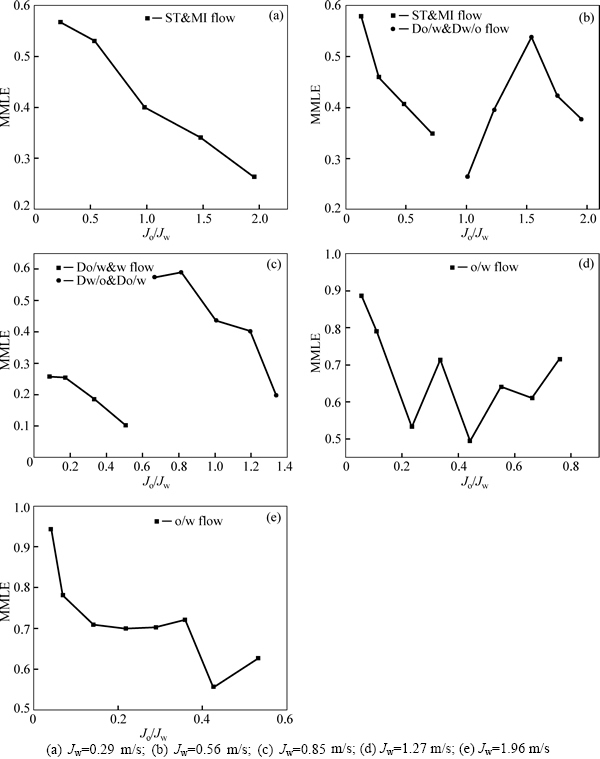
Fig. 6 Change of MMLE with oil superficial velocity at constant water superficial velocity:
Since the MMLE values of ST&MI flow and Dw/o&Do/w flow are similar, another feature to separate these two flow patterns is needed.
4.3 Correlation dimension of oil–water two-phase flow
The correlation dimension reflexes the degree of self-similarity of a dynamic system. Since the MMLE values of all the flow patterns are positive, the oil–water two-phase flow is verified to be a chaotic dynamic system that can be characterized with correlation dimensions. The change of flow pattern with water holdup is plotted in Fig. 7 against the correlation dimensions. The ST&MI flow has the highest correlation dimension, suggesting that the dual-continuous flow has high self-similarity flow structures. This self-similarity is mainly caused by the macro fluctuations caused by the wave between oil layer and the water layer, and the high frequency fluctuations by the oil droplets at the interface. The Do/w&w flow and the Dw/o&Do/w flow have similar value in correlation dimension, and the Do/w&w flow locates relatively below the Dw/o&Do/w flow. This reveals that the Do/w&w flow caused by the one dispersion layer and one continuous layer has more complex structures than the Dw/o&Do/w flow. The o/w flow has the lowest correlation dimension, indicating that the fluctuations of o/w flow is close to random due to the high velocity and low oil fraction. The oil droplets finely disperse in the water and flow with the turbulence without coalescence with each other.
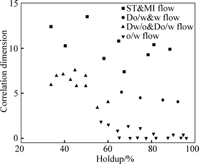
Fig. 7 Correlation dimension with different flow patterns
The change of correlation dimension with superficial velocity ratio Jo/Jw is illustrated in Fig. 8. The ST&MI flow has a relatively stable correlation dimension at water superficial velocity Jw=0.29 m/s. This reveals that the structure of ST&MI flow remains similar although water holdup increases. At Jw=0.56 m/s, the structure is broken by increasing oil fraction into the two-phase flow, which reduces the correlation dimension. The correlation dimension of Do/w&w flow increases with oil superficial velocity (Fig. 8(c)), because the flow structure becomes complex and ordered with more oil phases. This reveals that the oil droplets coalescence reduces the randomness of flow behaviors. When the flow pattern transits into the Dw/o&Do/w flow, the correlation dimension drops and then increases with oil superficial velocity, indicating that the formation of the dual dispersion flow structure will first introduce the random fluctuations into the oil–water two-phase system, and then the system becomes ordered when more oil phase is added. For o/w flow, the correlation dimension increases with oil superficial velocity when Jw=1.27 m/s, but remains stable when Jw=1.96 m/s. This phenomenon suggests that the oil droplets are easier to coalesce at low water superficial velocity, because the high dynamic energy and turbulence will easily break the coalescing process. The flow condition is more likely to be homogeneous at high superficial velocity.
4.4 Flow pattern separation with MMLE and correlation dimension
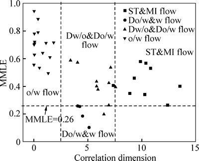
According to the above analysis, the MMLE and the correlation dimension characterize the flow structure in different manners, so they can jointly separate the flow patterns in an MMLE to correlation dimension map, as shown in Fig. 9. The o/w flow locates at the high MMLE and low correlation dimension part, due to its high disorder fluctuations and low self-similarity. The ST&MI flow locates at high correlation dimension part that separates from the Dw/o&Do/w flow, even though they overlap in MMLE. The Do/w&w flow has the lowest MMLE and its correlation dimension locates in between the o/w flow and the Dw/o&Do/w flow. There are some overlaps of the Do/w&w flow with the Dw/o&Do/w flow in both the MMLE and the correlation dimension, suggesting that the flow pattern transition occurs at these points, and these two flow patterns have similar structure, as demonstrated in Fig. 4. According to Fig. 9, three straight lines separate the flow patterns. The Do/w& flow can be separated from the other three flow patterns with MMLE<0.26. Besides, the o/w flow can be separated with correlation dimension lower than 2.5, and the ST&MI flow higher than 7.5. Finally, the Dw/o&Do/w flow is included with MMLE>0.26 and 2.5 4.5 Discussion One issue of the conductivity based sensing techniques is the change of conductivity in practical applications. This change can be compensated by using the relative change of the electrodes’ response in two-phase flow to that in the water-filled condition, as shown in Eq. (13). At the beginning of each group of experiments, the measurement when the pipe is filled with water is obtained, so the measurement in two-phase flow can be normalized to avoid the conductivity change between groups. Regular calibration can also be used in practical applications since the conductivity does not change rapidly from time to time. Fig. 8 Change of correlation dimension with water holdup at constant water superficial velocity: Fig. 9 Flow patterns with MMLE and correlation dimension Since ERT only provides valid measurements in water continuous flows, only the water continuous flow patterns are analyzed in the present work. Theoretically, the MMLE and correlation dimension can produce valid features even only one electrode functions, but the reliability and representatives under such a situation are questionable. Therefore, the above methods and results can be extended to oil continuous flow with an ECT system, which operates properly in oil continuous flow. The calculation process of the MMLE and the correlation dimension remains the same. This conductance/ capacitance dual-modality data analysis has been validated in the univariate data analysis [21]. Figure 9 is obtained only when the pipe diameter is 50 mm with specific oil and water, so the extendibility of the flow pattern boundaries needs further verification through more experiments. But the MMLE and correlation dimension map can remain valid since both of these two features reflect different dynamic characteristics of the oil–water flow systems. 5 Conclusions 1) A 16-variate vector is extracted from a high dimension measurement of one frame data of ERT. The 16-variate time-series is formed which consists of the simultaneous response of the phase distribution at each location where the corresponding electrode is installed. The multivariate maximum Lyapunov exponent is extracted from the 16-variate time-series to characterize and analyze the flow pattern change. The o/w flow is found to have the highest MMLE value due to its disorder characteristic at high flow velocity. The Do/w&w flow has the lowest MMLE while the Dw/o&Do/w flow and the ST&MI flow have similar MMLE. 2) To further separate the Dw/o&Do/w flow and the ST&MI flow, the correlation dimension of the 16-variate time-series is calculated, which reflects the self- similarity of a dynamic system. The flow patterns of oil– water two-phase flow can finally be separated on a MMLE versus correlation dimension map. The separation of Do/w& flow is achieved by MMLE, while the o/w flow, the Dw/o&Do/w flow and the ST&MI flow are segmented by correlation dimension. 3) Furthermore, the changes of MMLE and correlation dimension with oil superficial velocity at different water superficial velocities are also studied. The flow pattern transitions can be observed with a sudden change of both MMLE and correlation dimension, which demonstrates that these two features are sensitive to the change of flow structures in terms of disorder and self- similarity. References [1] ZHANG Jin-jun, LIU Xin. Some advances in crude oil rheology and its application [J]. Journal of Central South University, 2008, 15(s1): 288–292. [2] MORGAN R G, MARKIDES C N, ZADRAZIL I, HEWITT G F. Characteristics of horizontal liquid–liquid flows in a circular pipe using simultaneous high-speed laser-induced fluorescence and particle velocimetry [J]. International Journal of Multiphase Flow, 2013, 49: 99–118. [3] MORGAN R G, MARKIDES C N, HALE C P, HEWITT G F. Horizontal liquid–liquid flow characteristics at low superficial velocities using laser-induced fluorescence[J]. International Journal of Multiphase Flow, 2012, 43: 101–117. [4] LOVICK J, ANGELI P. Droplet size and velocity profiles in liquid–liquid horizontal flows [J]. Chemical Engineering Science, 2004, 59(15): 3105–3115. [5] ANGELI P, HEWITT G F. Drop size distributions in horizontal oil-water dispersed flows [J]. Chemical Engineering Science, 2000, 55(16): 3133–3143. [6] SHARIFI M, YOUNG B. Electrical resistance tomography (ERT) applications to chemical engineering [J]. Chemical Engineering Research and Design, 2013, 91(9): 1625–1645. [7] TAN Chao, DONG Feng, WU Meng. Identification of gas/liquid two-phase flow regime through ERT-based measurement and feature extraction [J]. Flow Measurement and Instrumentation, 2007, 18(5/6): 255–261. [8] KONG Ling-shuang, YANG Chun-hua, LI Jian-qi, ZHU hong-qiu, WANG Ya-lin. Generic reconstruction technology based on RST for multivariate time series of complex process industries [J]. Journal of Central South University, 2012, 19(5): 1311–1316. [9] TAN Chao, ZHAO Jia, DONG Feng. Gas-water two-phase flow characterization with electrical resistance tomography and multivariate multiscale entropy analysis [J]. ISA Trans, 2015, 55: 241–249. [10] CIGNETTI F, DECKER L M, STERGIOU N. Sensitivity of the Wolf’s and Rosenstein’s algorithms to evaluate local dynamic stability from small gait data sets [J]. Annuals of Biomedical Engineering, 2012, 40(5): 1122–1130. [11] LU Shan, WANG Hai-yan. Calculation of the maximal Lyapunov exponent from multivariate data [J]. Acta Physica Sinica, 2006, 55(2): 572–576. (in Chinese) [12] GRASSBERGER P, PROCACCIA I. Characterization of strange attractors [J]. Physical Review Letters, 1983, 50(5): 346–349. [13] WANG Ji-min, ZHOU Yuan-yuan, LAN Shen, CHEN Tao, LI Jie, YAN Hong-jie, ZHOU Jie-min, TIAN Rui-jiao, TU Yan-wu, LI Wen-ke. Numerical simulation and chaotic analysis of an aluminum holding furnace [J]. Metallurgical and Materials Transactions B, 2014, 45(6): 2194–2210. [14] DONG Feng, XU Cong, ZHANG Zhi-qiang, REN Shang-jie. Design of parallel electrical resistance tomography system for measuring multiphase flow [J]. Chinese Journal of Chemical Engineering, 2012, 20(2): 1–12. [15] TAKENS F. Detecting strange attractors in turbulence [M]// RAND D, YOUNG L S. Dynamical Systems and Turbulence. Springer Berlin Heidelberg, 1981: 366–381. [16] KIM H S, EYKHOLT R, SALAS J D. Nonlinear dynamics, delay times, and embedding windows [J]. Physica D, 1999, 127: 48–60. [17] GU Jian, CHEN Shu-yan. Nonlinear analysis on traffic flow based on catastrophe and chaos theory [J]. Discrete Dynamics in Nature and Society, 2014: 535167. [18] ROSENSTEIN M T, COLLINS J J, LUCA C J. A practical method for calculating largest Lyapunov exponents from small data sets [J]. Physica D, 1993, 65: 117–134. [19] TRALLERO J L, SARICA C, BRILL J P. A study of oil-water flow patterns in horizontal pipes [J]. SPE Production & Facilities, 1997, 12(3): 165–172. [20] XU Xiao-xuan. Study on oil–water two-phase flow in horizontal pipelines [J]. Journal of Petroleum Science and Engineering, 2007, 59(1/2): 43–58. [21] TAN Chao, LI Peng-fei, DAI Wei, DONG Feng. Characterization of oil-water two-phase pipe flow with a combined conductivity/ capacitance sensor and wavelet analysis [J]. Chemical Engineering Science, 2015, 134: 153–168. (Edited by YANG Bing) Foundation item: Projects(61227006, 61473206) supported by the National Natural Science Foundation of China; Project(13TXSYJC40200) supported by Science and Technology Innovation of Tianjin, China Received date: 2015-01-14; Accepted date: 2015-04-14 Corresponding author: DONG Feng, Professor, PhD; Tel: +86–22–27892055; E-mail:fdong@tju.edu.cn
Abstract: Oil–water two-phase flow patterns in a horizontal pipe are analyzed with a 16-electrode electrical resistance tomography (ERT) system. The measurement data of the ERT are treated as a multivariate time-series, thus the information extracted from each electrode represents the local phase distribution and fraction change at that location. The multivariate maximum Lyapunov exponent (MMLE) is extracted from the 16-dimension time-series to demonstrate the change of flow pattern versus the superficial velocity ratio of oil to water. The correlation dimension of the multivariate time-series is further introduced to jointly characterize and finally separate the flow patterns with MMLE. The change of flow patterns with superficial oil velocity at different water superficial velocities is studied with MMLE and correlation dimension, respectively, and the flow pattern transition can also be characterized with these two features. The proposed MMLE and correlation dimension map could effectively separate the flow patterns, thus is an effective tool for flow pattern identification and transition analysis.
