Trans. Nonferrous Met. Soc. China 26(2016) 736-746

Influence of material models on theoretical forming limit diagram prediction for Ti-6Al-4V alloy under warm condition

Nitin KOTKUNDE¹, Sashank SRINIVASAN¹, Geetha KRISHNA¹, Amit Kumar GUPTA¹, Swadesh Kumar SINGH²

1. Department of Mechanical Engineering, Birla Institute of Technology and Science-Pilani, Hyderabad Campus, Hyderabad 500078, Telangana, India;

2. Department of Mechanical Engineering, Gokaraju Rangaraju Institute of Engineering and Technology, Hyderabad 500072, Telangana, India

Received 26 February 2015; accepted 26 July 2015

Abstract:

Forming limit diagram (FLD) is an important performance index to describe the maximum limit of principal strains that can be sustained by sheet metals till to the onset of localized necking. It offers a convenient and useful tool to predict the forming limit in the sheet metal forming processes. In the present study, FLD has been determined experimentally for Ti-6Al-4V alloy at 400 °C by conducting a Nakazima test with specimens of different widths. Additionally, for theoretical FLD prediction, various anisotropic yield criteria (Barlat 1989, Barlat 1996, Hill 1993) and different hardening models viz., Hollomon power law (HPL), Johnson-Cook (JC), modified Zerilli–Armstrong (m-ZA), modified Arrhenius (m-Arr) models have been developed. Theoretical FLDs have been determined using Marciniak and Kuczynski (M-K) theory incorporating the developed yield criteria and constitutive models. It has been observed that the effect of yield model is more pronounced than the effect of constitutive model for theoretical FLDs prediction. However, the value of thickness imperfection factor (f₀) is solely dependent on hardening model. Hill (1993) yield criterion is best suited for FLD prediction in the right hand side region. Moreover, Barlat (1989) yield criterion is best suited for FLD prediction in left hand side region. Therefore, the proposed hybrid FLD in combination with Barlat (1989) and Hill (1993) yield models with m-Arr hardening model is in the best agreement with experimental FLD.

Key words:

Ti-6Al-4V alloy; yield criteria; hardening model; Marciniak and Kuczynski theory; forming limit diagram;

1 Introduction

Nowadays, titanium alloy is one of the most popular and commonly used alloys in automobile and aerospace industries. This is due to its attractive properties of high strength, light-mass, resistance to corrosion and low modulus [1]. Sheet metal forming processes, which are performed on these alloys, eliminate additional operations such as welding, machining and aid in developing parts with reduced mass, good mechanical properties at high production rates [2]. However, despite these lucrative properties, titanium alloys rank below steels in terms of total utility because of cost and formability issues at room temperature. The main reasons for poor formability are low ductility at room temperature due to the hexagonal close-packed structure and high degree of spring-back due to low elastic modulus [3]. The formability of these lightmass alloys can be greatly improved by warm forming. Elevated temperature forming results in decreased flow stress and increased ductility in the sheet, it allows deeper drawing and more stretching [4].

The forming limit diagram (FLD) is used as a design tool that quantitatively describes the formability limit of sheet metal forming processes. It is a graphical representation of the major strain and minor strain, plotted at the moment of the onset of necking [5]. Determining FLDs experimentally is generally a tedious, costly and elaborate process which naturally leads to great interest in developing and using numerical models and computational methods to predict them [6]. KEELER and BACKOFEN [7], the pioneers of FLDs, determined strains on the right hand side of the FLD. GOODWIN [8] extended the FLD by including negative minor strains. Consequently, considerable effort has been made to construct reliable forming limit prediction models [9]. The first realistic mathematical model has been developed by MARCINIAK and KUCZYNSKI (M-K) [10]. This model assumes a thickness imperfection in an infinite sheet metal, which is used to explain the necking behavior generally seen after significant deformation of materials. In order to relate stresses and strains present in the sheet, yield criterion and hardening rules along with the flow rule relations are required to be incorporated into the M-K model. The accuracy of the predicted FLD can be significantly influenced by the choice of yield criterion and hardening model [11].

The yield criterion proposed by HILL in 1948 [12] has been successfully applied for steel sheets over a long period and is still widely used. BUTUC et al [13] proposed the effect of different yield functions such as von Mises, Hill (1948) and Hill (1979) and Barlat (1996) with Swift and Voce model on forming limit diagram for AA6016-T4 alloy. Further attempts have been made to hypothesize more accurate prediction models for steel and aluminum alloy [14,15]. A few studies have been reported for the prediction of FLDs at elevated temperature as well [16]. However, with respect to titanium alloys, very few results have been reported [4,17]. LI e al [4] reported FLDs prediction of Ti-6Al-4V alloy using M-K theory along with von Mises yield criterion at elevated temperature. DJAVANROODI and DEROGAR [17] investigated FLDs experimentally using a special process of hydroforming deep drawing compared with finite element analysis using Hill-swift and NADDRG models. There is still a large void in exploring various other anisotropic yield criteria along with different hardening models for the FLD prediction of Ti-6Al-4V alloy.

The main objective of this work is to theoretically study the calculated FLDs for Ti-6Al-4V alloy at 400 °C using the M-K model and compare them with experimental results to measure the accuracy of the prediction model in consideration and understand the scope of improvement that still exists in this regard. The influences of various anisotropic yield criteria and hardening models on theoretical FLD prediction were studied. Here, the Barlat (1989), Barlat (1996) and Hill (1993) yield criteria with different hardening laws of Hollomon power law (HPL), Johnson-Cook (JC), modified Zerilli-Armstrong (m-ZA), modified Arrhenius (m-Arr) models were considered.

Table 1 Chemical composition of as-received Ti-6Al-4V sheet (mass fraction, %)

2 Experimental

2.1 Material properties

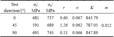
The composition of as-received Ti-6Al-4V alloy material is shown in Table 1. The uniaxial tensile tests were performed to determine various material constants which were required to build the yield criteria and hardening models that describe the material behavior in the plastic region. The samples used for the tensile tests were wire-cut using electro-discharge machining process for high accuracy and finish. The dimension of the specimens is according to ASTM E8/E8M-11 sub-size standard. The specimens were tested along three directions, with the tensile axis being parallel (0°), diagonal (45°), and perpendicular (90°) to the rolling direction of the sheet. The important material properties of strain hardening exponent (n), strain rate sensitivity (m), LANKFORD parameter (r), yield strength (σ_y), ultimate tensile strength (σ_u) and strength coefficient (K) were determined. Three samples were tested in each of the three directions and average values were reported to account for the scatter. The n value was determined from the regression of the load–displacement data obtained from the tensile tests, using Hollomon equation (1) [9]:

σ=Kεⁿ            (1)

The r value was evaluated based on the procedure mentioned by RAVIKUMAR [18]. The strain rate sensitivity (m) was calculated as continuous stress-strain curves at several different strain rates and compared the levels of stress at a fixed strain using modified Hollomon equation (Eq. (2)) [9]:

                                (2)

The calculated material properties for Ti-6Al-4V alloy at 400 °C are shown in Table 2.

Table 2 Material properties for Ti-6Al-4V alloy at 400 °C

2.2 Experimental forming limit diagram

Experimental FLD was plotted at 400 °C. Temperature higher than 400 °C increases the oxygen contamination in Ti-6Al-4V alloy and the material with oxygen becomes more brittle due to the formation of α-scale. Therefore, it is preferred to performing warm forming of Ti-6Al-4V alloy in an inert and protective environment. Considering the limitations of experimental facility at higher temperatures with inert environment, the FLD experiments were performed at 400 °C [2].

Experimental FLD was plotted based on Hecker’s simplified technique [19]. This procedure had three main stages, namely, grid marking on the sheet, punch stretching of the grid marked sheets to failure (onset of localized necking) and the measurement of strains on the deformed specimens. The sheet dimensions were chosen from 120 mm × 120 mm and one side was reduced by 10 mm for every specimen up to 30 mm. Circular grids of 5 mm in diameter were marked on the Ti-6Al-4V alloy sheet using electro-chemical etching process. The sheet samples were subjected to different states of strain, i.e., the uniaxial tension-compression zone, the plane strain and biaxial tension zone. For the repeatability of the experiments, three specimens were tested for each blank width and average values were considered for FLD prediction. Figure 1 shows the dimensions of specimens used for experimental FLD study.

The experimental setup used for FLD experimentation is shown in Fig. 2. It consists of a 20 t hydraulic press with two sets of furnaces. One heater is used for heating the sheet metal specimen, while the other is utilized for heating the lower die. Water is circulated around the die in a cooling capacity to attain the required temperature. This effective cooling arrangement maintains the temperature accuracy of±5 °C. A non-contact type pyrometer is used to measure the operating temperature. Based on a previous literature, molykote lubricant is used for FLD experiment under warm condition [20]. Punch speed is chosen as 30 mm/min and blank holding pressure is selected as 2% of the yield strength.

Grid marked specimens were kept at a particular temperature for 3-5 min to ensure uniform heating of the sheet. Then, stretching operation was performed at 400 °C. The resulting deformation led to the circular grids becoming ellipses. Figure 3 shows representative failed stretched specimens at 400 °C.

The major and minor strains determined along the two axes of the ellipses were measured using a travelling microscope with an inherent accuracy of 0.01 mm. The strains were estimated by measuring the deformation of the grid as near as possible to the fracture zone, neck zone and safe zone. Figure 4 shows strains obtained in fracture zone, neck zone and safe zone. For better accuracy of results, experiments have been performed three times and average major and minor strain values are considered. The forming limit curve (FLC) line has been drawn just below the necking strain limit of a material. The FLC has been considered as a safe formable limit of a material [9]. The FLC line is considered as a basis of comparison with theoretical FLDs.

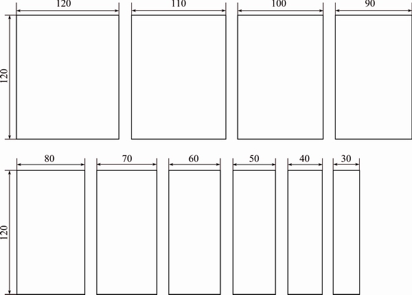
Fig. 1 Dimension details of specimen used for experimental FLD (unit: mm)

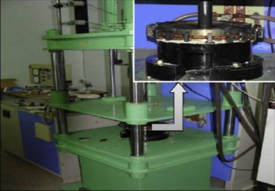
Fig. 2 Experimental test rig with enlarged view of die with induction furnace

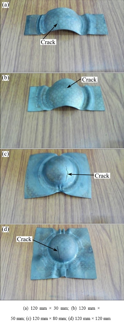
Fig. 3 Representative failed stretched specimens for Ti-6Al- 4V alloy at 400 °C

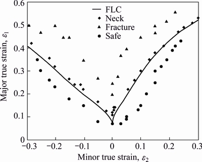
Fig. 4 Experimental FLD for Ti-6Al-4V alloy at 400 °C

3 Material models

3.1 Yield criteria

The transition from the elastic to plastic state occurs when a material reaches its yielding point. In multi-axial loading case, it is more difficult to define and predict the yielding behavior of a material. Therefore, mathematical relationships are crucial to describe the yield function. Commonly, there is a relation between the principal stresses in multi-axial loading case and yield stress in uniaxial case. The generalized equation for yield criteria can be expressed by Eq. (3):

F(σ₁, σ₂, σ₃, σ_y)=0                             (3)

where σ₁, σ₂ and σ₃ are the principal stresses and σ_y is the yield stress obtained from a simple tension test [9]. Equation (3) indicates the mathematical description of a surface in the three dimensional space of the principal stresses generally called the yield locus. Generally, the sheet metal analysis is considered as a plane stress problem. Therefore, in the case of plane stress (e.g., σ₃=0), the yield surface reduces to a curve in the plane of the principal stresses σ₁ and σ₂. The expression of the yield function is established on the basis of some phenomenological considerations concerning the transition from the elastic to the plastic state. The most widely used yield criteria for isotropic materials were proposed by Tresca (“maximum shear stress criterion”) and Huber–von Mises (“strain energy criterion”) [17]. However, these two popular yield criteria do not take into account of the anisotropy of sheet metal. Therefore, these criteria were not very well suited for sheet metal forming analysis [12]. In the present study, Barlat (1989), Barlat (1996) and Hill (1993) yield criteria were considered for theoretical FLD prediction.

3.1.1 Barlat (1989) yield criterion

The extension of the Hosford theory [21] to incorporate effects in materials exhibiting normal anisotropy was proposed by Barlat and Richmond. For transversely isotropic material, the Barlat (1989) criterion is mathematically a variation of Hill (1948) in which the yield function exponent m takes the value of 2. The exponent is crystallographic dependent wherein it takes 6 or 8 accordingly whether the structure is BCC or FCC [22]. Barlat (1989) yield criterion is expressed as Eq. (4).

f=a|k₁+k₂|^M+a|k₁-k₂|^M+c|2k₂|^M=2σ^a        (4)

where M is an integer exponent, k₁ and k₂ are invariants of the stress tensor and are obtained from

                              (5)

               (6)

and a, c, h and p are material parameters determined by

              (7)

                              (8)

where r₀ is the anisotropic coefficient in rolling direction of sheet and r₉₀ is the anisotropic coefficient perpendicular to the rolling direction.

The p value can be found by iterative procedure. The detailed procedure to determine the material constants was mentioned by previous work done by BARLAT and RTCHMOND [22]. The calculated material parameters for Ti-6Al-4V alloy at 400 °C are shown in Table 3. Barlat (1989) yield locus for Ti-6Al-4V alloy at 400 °C is shown in Fig. 5. The normalized principal stresses have been considered to plot the yield locus.

Table 3 Material constants for Barlat (1989) yield criterion at 400 °C

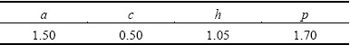
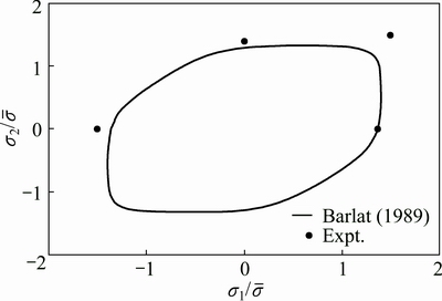
Fig. 5 Yield locus of Barlat (1989) yield criterion at 400 °C

Barlat yield criteria are popularly used in industry because of the ease of determining the material constants by only using uniaxial tensile test [9]. Since, most metal forming operations are carried out under biaxial states of stress; the stress–strain formability parameters obtained by uniaxial tensile testing are inadequate. Implementation of further yield criteria like Barlat (1996), Hill (1993) requires biaxial experimental properties. In the present study, biaxial data for Ti-6Al-4V alloy at 400 °C were taken from previous work done by ODENBERGER et al [23]. Table 4 indicates biaxial material properties and compressive yield strength for Ti-6Al-4V alloy at 400 °C.

3.1.2 Barlat (1996) yield criterion

Barlat (1996) yield function is expressed as

f=α_x|S_y-S_z|^a+α_y|S_z-S_x|^a+α_z0|S_x-S_y|^a=2^a                  (9)

where  is the equivalent stress, a is the material parameter, and S_i corresponds to principal values of Cauchy stress deviator.

                      (10)

The detailed procedure for determining the constants was mentioned by previous work done by KOTKUNDE et al [24]. The calculated material constants for Ti-6Al-4V alloy at 400 °C are shown in Table 5. Yield locus for Barlat (1996) for Ti-6Al-4V alloy at 400 °C is shown in Fig. 6.

Table 4 Biaxial material properties and compressive yield strength for Ti-6Al-4V alloy [23]

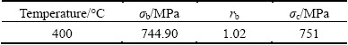
Table 5 Material constants for Barlat (1996) yield criterion at 400 °C

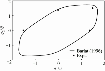
Fig. 6 Yield locus of Barlat (1996) yield criterion at 400 °C

3.1.3 Hill (1993) yield criterion

Hill (1993) improved the plastic behavior model of textured sheet metals, especially when complex loads were applied along the planar orthotropic axes. This criterion accounts for both “anomalous behavior of first order” and the “anomalous behavior of second order” [25]. These constraints set behaviours are satisfied by the polynomial (Eq. (11)). However, this is valid for stress states in the first quadrant (biaxial tension) only, which is the most relevant for thin sheet metals:

+        (11)

where c is given by

                     (12)

p and q are calculated with the normality condition of the strain rate tensor to the yield surface applied to function at the intersection with the coordinate axes as Eq. (13):

  (13)

The detailed procedure for constant determination is mentioned by previous work done by SIGUANG et al [25]. The calculated material constants for Hill (1993) are shown in Table 6. Hill (1993) yield locus for Ti-6Al-4V alloy at 400 °C is shown in Fig. 7.

Table 6 Material constants for Hill (1993) yield criterion at 400 °C

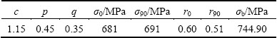
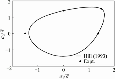
Fig. 7 Yield locus of Hill (1993) yield criterion at 400 °C

Figure 5 shows yield locus using Barlat 1989 yield criterion for Ti-6Al-4V alloy at 400 °C. It is clear from the locus that even though it predicts the uniaxial tensile region in rolling direction accurately, it is unable to predict the uniaxial compression and biaxial tension states. One major advantage of these criteria is the easy calculation of parameters which depend only on uniaxial tensile test experiments [24]. On the other hand, locus obtained by Barlat (1996) yield function shown in Fig. 6 nearly approximates the experimental data points for Ti-6Al-4V alloy. But the prediction capability of Barlat (1996) yield criterion is still poor. It may be because this yield criterion does not consider tension-compression asymmetry (Bauschinger effect) [9]. Figure 7 shows the yield locus for Hill (1993) yield criterion for Ti-6Al-4V alloy at 400 °C. It can be seen from Fig. 7 that the prediction capability of Hill (1993) yield criterion is very good in the region of uniaxial tension and biaxial state region. It also takes into account of tension-compression asymmetry. However, the prediction is slightly poor in uniaxial compression region. Based on the comparison of yield locus, Hill 1993 yield criterion is best suited for Ti-6Al-4V alloy at 400 °C.

3.2 Hardening models

The M-K model which is used in this study to predict FLDs requires the usage of stress-strain relations in the form of hardening models. The final outcome of the theoretical FLD prediction is based on strain values, therefore, hardening models play a major role in the accuracy of the predictions [26]. In this study, Hollomon power law (HPL), Johnson-Cook (JC), modified Zerilli–Armstrong (m-ZA), modified Arrhenius (m-Arr) are considered in M-K theory for the theoretical prediction of FLD. For determining various constants of hardening model, tensile test experiments were performed from 50 to 400 °C at an interval of 50 °C with constant strain rates of 1×10^-5, 1×10^-4, 1×10^-3 and 1×10^-2 s^-1. Each test was performed three times and average flow stress values were considered for flow stress prediction. The detail procedure for determining the constants of hardening models was mentioned in previous work done by KOTKUNDE et al [3,27].

Correlation coefficient (R) is a commonly used statistical tool which provides information on the strength of linear relationship between the experimental and predicted values. Although the value of R might be high, it is not necessary that the performance of the model is high, as the model might have a tendency to be biased towards higher values or lower values of the data [28]. Hence, average absolute error (Δ), which is computed through a term by term comparison of the relative error, is an unbiased statistics for measuring the predictability of the model. Therefore, the prediction capability of constitutive models was assessed by correlation coefficient (R), average absolute error (Δ) and its standard deviation (S). Table 7 shows capability of various hardening models based on statistical measures. The representative flow stress predictions using various hardening models are shown in Fig. 8.

Table 7 Comparison of various hardening models based on statistical measures

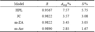
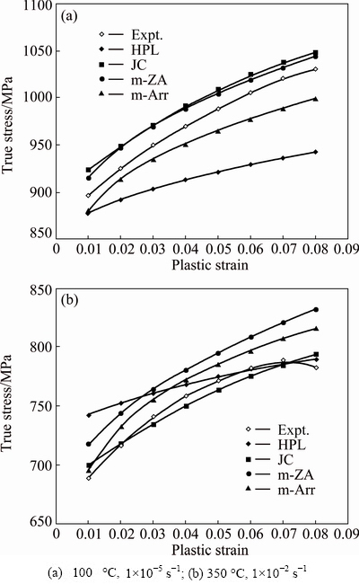
Fig. 8 Representative flow stress prediction using various hardening model under different conditions

It can be seen from Table 7 and Fig. 8 that, m-Arr model is more accurate compared with other models. Considering the correlation coefficient (R), all the models show very high degree of goodness of fit as the R value is above 0.95. However, R may be biased towards lower or higher value. Therefore, average absolute error (Δ) and its standard deviation (S) are used to check the accuracy of the predictions [28]. Considering all the statistical measures, HPL model has more deviation than other hardening models. Among all the considered models, m-Arr model is the best in agreement for flow stress prediction.

4 Marciniak-Kuczynski (M-K) model for FLD prediction

M-K model assumes an initial thickness imperfection in the geometry of the sheet in the form of a groove across the width of the sheet. A Cartesian coordinate system is aligned with the symmetry axes: x-axis is along the rolling direction (RD), and y-axis is along the transverse direction (TD). Figure 9 shows the sheet along with the groove that is assumed to exist. The zone outside the groove is considered as zone A and the groove region is considered as zone B.

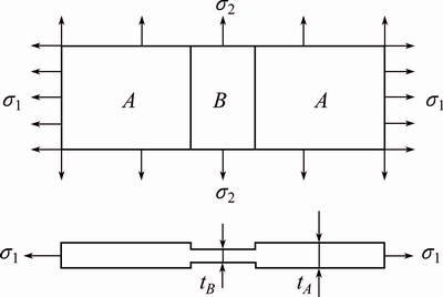
Fig. 9 Geometric imperfection of Marciniak-Kuczinsky (M-K) model

This initial imperfection can be defined by a thickness ratio:

                                 (14)

where  and  are the initial thicknesses of zones A and B, respectively, and f₀ is an inhomogeneity parameter of the M-K model. The boundary of the sheet (assumed to be far away from the groove) is subjected to continuous proportional straining parallel to the symmetry axes.

                               (15)

where ε_x and ε_y are components of strain along the coordinate axes. The ε_x component of the strain is referred to as the major strain, whereas ε_y is called the minor strain. The value of f₀ is varied until the predicted FLD curve agrees best with the experimental curve under the plane strain condition, i.e., for ρ=0. As the strain at the boundary increases, the thickness of zone B reduces faster than that of region A. Hence, it has to incur higher strains than those in zone A. The moment when region B has undergone deformation is drastically higher than that of region A, the material will give in, which is signified by the onset of necking. The failure criterion is

                                  (16)

where  and  denote the equivalent strains in the regions A and B, respectively. While implementing the M-K model computationally, the value of N attained when the sheet has failed should be very small. This means that region B has deformed much more seriously than region A, which is nothing but the formability limit of the material. Generally, the value of N is chosen between 0.15 and 0.20. In this study, the value of N is chosen to be 0.15. Thus, the criterion used is that region B should deform approximately 7 times more than region A for the sheet to reach its forming limit.

The ratios of principal stresses and strains are defined as

                      (17)

where x is the rolling direction and y is the transverse direction. The effective stress and strain are defined as

              (18)

The associative flow rule is given by

                              (19)

Using the associative flow rule and the constant volume condition given by Eq. (20), dε_x, dε_y and dε_z are obtained.

dε_x+dε_y+dε_z=0                               (20)

The M-K model incorporates a compatibility condition which states that regions A and B undergo equal straining in the transverse direction denoted by y axis:

                                 (21)

Furthermore, during the forming process, the sheet metal will always be under static equilibrium. This is captured by the force balance:

            (22)

where C is the function representing the required constitutive model/hardening law,  and f=t_A/t_B, and t_A and t_B denote the instantaneous thicknesses of regions A and B, respectively. This ratio can be obtained by

                         (23)

During the procedure to plot the FLD using M-K model, the value of f₀ is arbitrary. This value is varied in a range of 0.85 to 0.999, to ensure that at some values the predicted FLD matches the experimental results under the plain strain condition. The value of ρ is varied from -0.45 to 0.95 to get all the points on the FLD. The variation of ρ is done so as to find the forming limit along different strain paths that the sheet metal can possibly endure during the actual forming process. Small strain increments of  are imposed in the groove region. Iteratively, assuming a value for, the values of , ,  and  are computed and the equality of the force balance equation is checked. If the equality is satisfied, the ratio dε_A/dε_B is calculated. Further, if this ratio is lower than the limit of 0.15 that has been levied on the constant N, the process is stopped and the most recent values of the major and minor strains of region A are taken to denote the coordinates of a point lying on the FLD. If the ratio dε_A/dε_B is less than 0.15, additional increments of strain are imposed on region B till the straining limit is achieved. Figure 10 shows flow chart for theoretical FLD prediction using M-K theory.

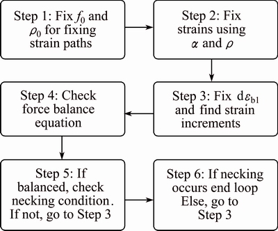
Fig. 10 Flow chart for theoretical FLD prediction

5 Results and discussion

As described previously, the procedure used to predict FLDs using the M-K theory will have to assume a value for parameter f₀, which denotes the initial thickness ratio of regions A and B. The fact that the M-K model uses this initial thickness defect to explain the forming limit makes this parameter a crucial one [16]. Furthermore, the value of f₀ can take any value based on thickness of the sheet, surface quality of sheet, grain size and material properties [25]. This makes it impossible to judge which will ensure correct predictions of the FLD. This is ensured by matching the FLDs with experimentally obtained forming limits under the plane strain condition. The value of f₀ which matches the experimental results will be used to make the predictions [16].

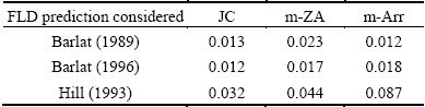
For all combinations of yield criteria and hardening models considered in this study, the value of f₀ is varied in a wide range. The final values used for theoretical FLDs prediction are listed in Table 8. It is evident from Table 8 that the hardening models seem to be the only factor that determines the value of this parameter. This is further strengthened by the fact that this is not restricted to one class of yield criteria. This observation related to f₀ value is a very intriguing and not so easily controvertible fact.

Table 8 Final f₀ values used for theoretical FLDs predictions

The effect of changing the value of f₀ for a particular combination of yield criterion and hardening rule also follows a general trend. As the value of f₀ decreases, the FLD’s shape remains the same but the whole plot is displaced in the negative y direction. Figure 11 shows such a representative situation. The f₀ value denotes the extent to which the groove region is thinner than the normal sheet region. The lower the value of f₀ is, the thinner the groove region will be. This will make the groove more prone to necking as a result of increase in deformation rate in comparison to a thicker groove. This results in lower forming limits, which is characterized by the FLD traversing in the negative y direction.

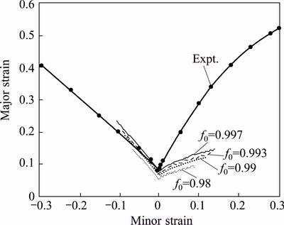
Fig. 11 Variation of f₀ value for FLD prediction

The final predictions of theoretical FLDs using various yield criteria with variation of hardening models are shown in Figs. 12-14. From a visual inspection of the plot, it can be seen that the predicted FLDs do not seem to vary much with change in hardening rule for a particular yield criterion. This was further analyzed by calculating the Fréchet distances between the predictions, the results of which are given in Table 9. The Fréchet distance is a measure of similarity between curves P and Q. It is defined as the minimum cord-length sufficient to join a point traveling forward along P and one traveling forward along Q, although the rate of travel for either point may not necessarily be uniform [29]. This correlation study has been done by assuming the HPL prediction as the base case and finding the similarity between this and the FLDs predicted by the other hardening models. This gives a more quantitative reasoning of the above conclusion.

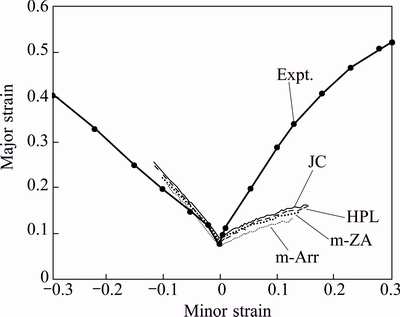
Fig. 12 Theoretical FLD using Barlat (1989) yield criterion with various hardening models

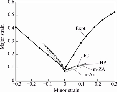
Fig. 13 Theoretical FLD using Barlat (1996) yield criterion with various hardening models

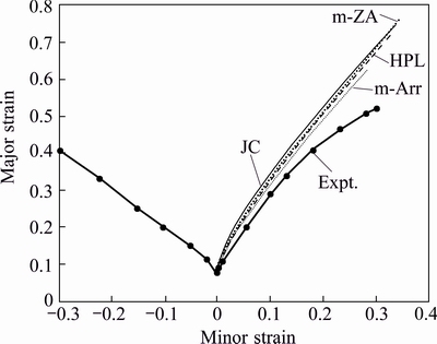
Fig. 14 Theoretical FLD using Hill (1993) yield criterion with various hardening models

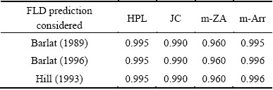
Table 9 Fréchet distance between FLD predictions

It can be seen from Figs. 12 and 13 that Barlat (1989) and Barlat (1996) yield criteria predict the left part of FLD (uniaxial state stress region) better than the right part (biaxial stress state region). This effect of poor prediction of biaxial region can be seen in the yield loci of these criteria as well. However, Barlat (1989) model is slightly more accurate than the Barlat (1996) model.

Hill (1993) yield criterion only involves two principal stresses which act along in-plane orthotropic directions. Based on the previous study done by SIGUANG et al [25], it is more suitable for the analysis of the right-hand side of forming limit diagram. The yield criterion needs to include shear stress in order to analyze the left-hand side of FLDs. However, this criterion predicts the right half of the curve more accurately than any other yield criteria considered. It can also be seen from Fig. 14 that the forming limit curves developed using Hill (1993) and modified Arrhenius (m-Arr) constitutive models predict the best among all the hardening models considered. It can be also observed that, yield criterion effect is more predominant in theoretical FLDs prediction than the hardening models. However, the effect of hardening models is limited to f₀ value.

Another interesting observation was the accuracy of the predictions with respect to the experimental results. The Barlat (1989) predictions were accurate for the negative minor strains but were very poor in the positive major strain regions. The Hill (1993) model, on the other hand, was accurate in the positive minor strain region. This made for an interesting idea of combining the negative region of the Barlat (1989) model and the positive region prediction of the Hill (1993) model. The resulting hybrid prediction of the FLD is shown in Fig. 15.

6 Conclusions

1) The Hill (1993) yield criterion best predicts the yielding of Ti-6Al-4V alloy at 400 °C. Moreover, m-Arr hardening model is best in agreement for flow stress prediction.

2) The variation of FLD due to the variation of the yield models for a particular hardening model is more pronounced than that of FLD due to the hardening models for a particular yield criterion. Moreover, the hardening model does not affect the FLD apart from determining the forming limit under the plane strain condition, due to the influence on the value of f₀.

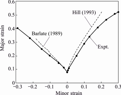
Fig. 15 Hybrid prediction of FLD with Barlat (1989) and Hill (1993) criteria

3) The Barlat class yield criteria predict the FLD best in the negative minor strain region while the Hill (1993) yield criterion is more accurate in the positive minor strain region of the FLD. Among the Barlat models considered, the Barlat (1989) is more accurate than the Barlat (1996) yield model. The trends in the FLD predicted by the two models however remain the same.

4) A hybrid FLD using Barlat (1989) (left side region) and Hill (1993) (right side region) yield models with m-Arr hardening model is the best to predict theoretical necking limit for Ti-6Al-4V alloy at 400 °C. The resulting FLD is proved to be in very close agreement with experimental results.

5) Future work involves FLD predictions using other anisotropic yield criteria.

Acknowledgment

The financial support received for this research work from Department of Science and Technology (DST), Government of India, SERB-DST, SR/FTP/ETA- 0056/2011 is gratefully acknowledged.

References

[1] BEAL D J, BOYER R, SANDERS D. ASM handbook B [M]. Ohio: ASM International, 2006.

[2] KOTKUNDE N, DEOLE A, GUPTA A K, SINGH S K, BALU A. Failure and formability studies in warm deep drawing of Ti-6Al-4V alloy [J]. Materials and Design, 2014, 60: 540-547.

[3] KOTKUNDE N, HANSOGE N K, PURANIK P, GUPTA A K, SINGH S K. Microstructure study and constitutive modeling of Ti-6Al-4V alloy at elevated temperatures [J]. Materials and Design, 2014, 54: 96-103.

[4] LI Xiao-qiang, GUO Gui-qiang, XIAO Jun-jie, SONG Nan, LI Dong-sheng. Constitutive modeling and the effects of strain-rate and temperature on the formability of Ti-6Al-4V alloy sheet [J]. Materials and Design, 2014, 55: 325-334.

[5] KURUKURI S, BOOGAARD A H, MIROUX A G, HOLMEDAL B. Warm forming simulation of Al-Mg sheet [J]. Journal of Materials Processing Technology, 2009, 209: 5636-5645.

[6] NAKA, T, YOSHIDA F. Deep drawability of type 5083 aluminum–magnesium alloy sheet under various conditions of temperature and forming speed [J]. Material Processing Technology, 1999, 89-90: 19-23.

[7] KEELER S P, BACKOFEN W A. Plastic instability and fracture in sheets stretched over rigid punches [J]. Trans of ASM, 1963, 56: 25-48.

[8] GOODWIN G M. Application of strain analysis to sheet metal forming problems in the press shop [J]. Metallurgica, 1968, 8: 767-774.

[9] BANABIC D. Sheet metal forming processes [M]. Heidelberg: Springer, 2010.

[10] MARCINIAK M, KUCZYNSKI S. Determination of the forming limit diagram for Al 3105 sheet [J]. Materials Processing Technology, 2003, 141: 138-142.

[11] DASAPPA P, KAAN I, MISHRA R. The effects of anisotropic yield functions and their material parameters on prediction of forming limit diagrams [J]. International Journal of Solids and Structures, 2012, 49: 3528-3550.

[12] HILL R. A theory of the yielding and plastic flow of anisotropic metals [J]. Proceedings of the Royal Society of London (Series A): Mathematical and Physical Sciences, 1948, 193: 281-297.

[13] BUTUC M C, GRACIO J J, da ROCHA A B. A theoretical study on forming limit diagrams prediction [J]. Material Processing Technology, 2003, 142: 714-724.

[14] FANG G, LIU Qing-jun, LEI Li-ping, ZENG Pan. Comparative analysis between stress- and strain-based forming limit diagrams for aluminum alloy sheet 1060 [J]. Transactions of Nonferrous Metals Society of China, 2012, 22(2): 343-349.

[15] NARAYANASAMY R, NARAYANAN C. Experimental analysis and evaluation of forming limit diagram for interstitial free steels [J]. Materials and Design, 2007, 28: 1490-1512.

[16] SANSOT P, BARLAT F, UTHAISANGSUK V, SURANUNTCHAIS. Experimental and theoretical formability analysis using strain and stress based forming limit diagram for advanced high strength steels [J]. Materials and Design, 2013, 51: 756-766.

[17] DJAVANROODI F, DEROGAR A. Experimental and numerical evaluation of forming limit diagram for Ti6Al4V titanium and Al6061-T6 aluminum alloys sheets [J]. Materials and Design, 2010, 31: 4866-4875.

[18] RAVIKUMAR D. Formability analysis of extra-deep drawing steel [J]. Materials Processing Technology, 2002, 130-131: 31-41.

[19] HECKER S S. Simple technique for determining forming limit curves [J]. Sheet Met Ind, 1975, 52: 671-675.

[20] SINGH S K, RAVI KUMAR D. Effect of process parameters on product surface finish and thickness variation in hydro-mechanical deep drawing [J]. Material Processing Technology, 2008, 204: 169-178.

[21] HOSFORD W F. A generalized isotropic yield criterion [J]. Applied Mechanics, 1972, 39: 607-609.

[22] BARLAT F, RICHMOND O. Prediction of tricomponent plane stress yield surfaces and associated flow and failure behaviour of strongly textured FCC polycrystalline sheets [J]. Materials Science and Engineering A, 1987, 91: 15-29.

[23] ODENBERGER E L, SCHILL M, OLDENBURG M. Thermo-mechanical sheet metal forming of aero engine components in Ti-6Al-4V. Part 2: Constitutive modelling and validation [J]. Material Forming, 2013, 6(3): 403-416.

[24] KOTKUNDE N, DEOLE A, GUPTA A K, SINGH S K. Experimental and numerical investigation of anisotropic yield criteria for warm deep drawing of Ti-6Al-4V alloy [J]. Materials and Design, 2014, 63: 336-344.

[25] SIGUANG X U, KLAUS J, WEINMANN. Prediction of forming limit curves of sheet metals using Hill’s 1993 user-friendly yield criterion of anisotropic materials [J]. Mechanical Sciences, 1998, 40(9): 913-925.

[26] LIN Y C, CHEN X M. A critical review of experimental results and constitutive descriptions for metals and alloys in hot working [J]. Materials and Design, 2011, 32: 1733-1759.

[27] KOTKUNDE N, DEOLE A, GUPTA A K, SINGH S K. Comparative study of constitutive modeling for Ti-6Al-4V alloy at low strain rates and elevated temperatures [J]. Materials and Design, 2014, 55: 999-1005.

[28] GUPTA A K, KRISHNAMURTHY H N, SINGH Y, PRASAD K M, SINGH S K. Development of constitutive models for dynamic strain aging regime in austenitic stainless steel 304 [J]. Materials and Design, 2013, 45: 616-627.

[29] ALT H, GODAU M. Computing the fréchet distance between two polygonal curves [J]. Computational Geometry & Applications, 1995, 5(1-2): 75-91.

材料模型对高温Ti-6Al-4V合金理论成形极限图预测的影响

Nitin KOTKUNDE¹, Sashank SRINIVASAN¹, Geetha KRISHNA¹, Amit Kumar GUPTA¹, Swadesh Kumar SINGH²

1. Department of Mechanical Engineering, Birla Institute of Technology and Science-Pilani, Hyderabad Campus, Hyderabad 500078, Telangana, India;

2. Department of Mechanical Engineering, Gokaraju Rangaraju Institute of Engineering and Technology, Hyderabad 500072, Telangana, India

摘  要：成形极限图是一种用来描述使板材不发生局部颈缩所需最大主应变的重要图形。它是一种预测板材变形过程中变形极限的方便、有效的工具。本研究中，在400 °C和不同样品宽度的条件，通过Nakazima实验得到了Ti-6Al-4V合金的成形极限图。此外，为了使用成形极限图对材料参数进行理论预测，提出了不同的各向异性屈服准则(Barlat 1989, Barlat 1996, Hill 1993)和不同的硬化模型(Hollomon幂定律、Johnson-Cook(JC)模型、改进的Zerilli-Armstrong (m-ZA)和Arrhenius (m-Arr)模型)。结合所提出的屈服准则和本构模型，通过Marciniak和Kuczynski (M-K)理论确定了Ti-6Al-4V合金的成形极限图。结果表明：屈服模型对材料成形极限图的影响大于本构模型的影响。然而，材料的厚度缺陷系数(f₀)与其硬化模型密切相关。Hill(1993)屈服准则最适合于成形极限图右边区域的预测，而Barlat(1989)屈服准最适合于成形极限图左边区域的预测。由于所得到的混合理论成形极限图兼具Barlat(1989)和Hill(1993)屈服模型和m-Arr硬化模型的优点，因此，它与实验得到的成形极限图吻合很好。

关键词：Ti-6Al-4V合金；屈服准则；硬化模型；Marciniak-Kuczynsk理论；成形极限图

(Edited by Wei-ping CHEN)

Corresponding author: Nitin KOTKUNDE; Tel: +91-9010451444; Fax: +91-40-66303998; E-mail: nitink@hyderabad.bits-pilani.ac.in

DOI: DOI:10.1016/S1003-6326(16)64140-7

Abstract: Forming limit diagram (FLD) is an important performance index to describe the maximum limit of principal strains that can be sustained by sheet metals till to the onset of localized necking. It offers a convenient and useful tool to predict the forming limit in the sheet metal forming processes. In the present study, FLD has been determined experimentally for Ti-6Al-4V alloy at 400 °C by conducting a Nakazima test with specimens of different widths. Additionally, for theoretical FLD prediction, various anisotropic yield criteria (Barlat 1989, Barlat 1996, Hill 1993) and different hardening models viz., Hollomon power law (HPL), Johnson-Cook (JC), modified Zerilli–Armstrong (m-ZA), modified Arrhenius (m-Arr) models have been developed. Theoretical FLDs have been determined using Marciniak and Kuczynski (M-K) theory incorporating the developed yield criteria and constitutive models. It has been observed that the effect of yield model is more pronounced than the effect of constitutive model for theoretical FLDs prediction. However, the value of thickness imperfection factor (f₀) is solely dependent on hardening model. Hill (1993) yield criterion is best suited for FLD prediction in the right hand side region. Moreover, Barlat (1989) yield criterion is best suited for FLD prediction in left hand side region. Therefore, the proposed hybrid FLD in combination with Barlat (1989) and Hill (1993) yield models with m-Arr hardening model is in the best agreement with experimental FLD.