
J. Cent. South Univ. (2012) 19: 1482-1487
DOI: 10.1007/s11771-012-1165-4![]()
Modeling of radiative properties of metallic microscale rough surface
WANG Ai-hua(������)1, 2, CAI Jiu-ju(�̾ž�)1
1. School of Materials and Metallurgy, Northeastern University, Shenyang 110819, China;
2. Department of Mechanical and Aerospace Engineering, Florida Institute of Technology, Melbourne 32901, USA
? Central South University Press and Springer-Verlag Berlin Heidelberg 2012
Abstract:
The radiative properties of a gold surface with one-dimensional Gaussian random roughness distribution were obtained with the finite-difference time-domain (FDTD) method and the recursive convolution treatment of the Drude Model. The bi-directional reflection distribution function (BRDF) for both TM mode and TE mode were obtained and compared with the highly accurate experimental data from the earlier work. The incident wavelength varies from 1.152 ��m to 3.392 ��m and incident angle is at 30��-70��, respectively. The results show that, the predicted values and experimental results are in good agreement. The highly specular peak in the BRDF is reproduced in the numerical simulations, and the increase of the TM mode BRDF is found to be attributed to the effect of a variation in the optical constant at the incident wavelength period.
Key words:
1 Introduction
Electromagnetic wave scattering from patterned or random roughness surfaces and coatings is of fundamental and practical interests to many disciplines, e.g. remote sensing, surface optics [1], thermal control [2], and wafer thermal processing [3]. It presents great theoretical challenges due to the large degrees of freedom in these systems and the need to include multiple scattering effects accurately. In recent years, rapid advances in computer modeling have opened new approaches, for example, finite difference, finite element, Monte Carlo simulations, in the numerical analysis of random media scattering [4]. Numerical simulations allow us to solve the Maxwell��s equations exactly without the limitations of analytical approximations, whose regimes of validity are often difficult to assess.
Several theoretical treatments have been developed to understand light scattering from very rough surfaces, for example, the ray tracing method [5] and the integral equation method of solving Maxwell��s equations [6]. Due to difficulties in computing higher-order terms and in the solution convergence, perturbation series have been limited to weakly rough surfaces. Geometric ray tracing is limited to roughness being larger than the incident wavelength, so the wave interference effect can be neglected [7]. The finite-difference time-domain (FDTD) method produced highly accurate solutions to understand the light scattering process of microscale random roughness in different surfaces. For the metallic surfaces, the original FDTD equations have to be modified to ensure solution convergence. This requires the use of the time-domain electrical properties to revise the difference equations.
It is not easy to experimentally produce microscale random roughness surfaces that follow the Gaussian relation requirement in the surface height distribution and the height correlation function. KNOTTS and O��DONNELL [8] used a photoresist method to produce a set of well defined one-dimensional Gaussian roughness gold surfaces. They measured the coherent and incoherent components of the polarized intensities scattered from the surfaces. Some of their experimental results are used in this work to compare with the FDTD predictions. The bi-directional reflection distribution function (BRDF) is of particular interest in this work.
2 Theoretical fundamentals
2.1 Finite-difference time-domain method
For a two-dimensional geometry, FDTD form of TE (normal polarization) set of the Maxwell��s equations can be written for the incident plane, i.e., the x-y plane that contains Ez, Hx, and Hy. The finite difference form of TM (parallel polarization) equation set can be written similarly. The details are readily available in the original work of YEE [9] and are not. In the discretized mesh of the computational domain, E and H are spatially shifted by 1/2 space increment, and the calculation of them is temporally shifted by 1/2 time increment, so that all unknown variables at any time step can be calculated based on the variables at the previous half and full-time step status. With the second-order central difference scheme, the TE mode Maxwell��s equations in 2D can be expressed as
![]()
![]()
![]() (1a)
(1a)
![]()
![]() (1b)
(1b)
![]()
![]() (1c)
(1c)
where the superscript of the field components stands for time step, the subscript represents the spatial node location; �� is the permittivity; �� is the permeability; �� is the conductivity. Note that in Eq. (1), �� and ��* are set to be zero for dielectric and non-magnetic materials. According to YEE��s notation, a spatial point in a Cartesian coordinate is written as (i, j)=(i?x, j?y). ?x and ?y are the lattice space increments in the x and y coordinate directions, respectively, and i and j are integers.
If the interface of different materials is parallel to one of the coordinate axes, continuity of tangential E and H is naturally maintained; the algorithm itself is divergence-free in the absence of electric and magnetic charge; the time-stepping algorithm is nondissipative, which means that EM wave propagating within the mesh will not decay due to the algorithm itself. All these results make YEE��s algorithm a robust method in solving EM field issues.
2.2 Recursive convolution treatment of Drude model
The Maxwell-Ampere law in the Maxwell��s equations is
![]() (2)
(2)
where all quantities with a ��^�� indicate complex number, e.g., ![]() . Assume a time harmonic incident field:
. Assume a time harmonic incident field:
![]() (3)
(3)
Then, Eq. (2) becomes
![]() (4)
(4)
Substituting the complex forms of ![]() and
and ![]() into Eq. (4), we have
into Eq. (4), we have
![]()
![]()
![]() (5)
(5)
To distinguish from ��, the dielectric function or dielectric constant is expressed as ![]() ��e and ��e are equivalent properties and are used in the FDTD equations (Eq. (1)). When n2�C��2=?'=��e/��o<0, the FDTD code cannot converge because the coefficient of the first terms on the right hand side of Eq. (1) and similar difference equations are greater than 1 and the second term is smaller than the first term. This means that Ez or H field components could have non-steady or large oscillations through time stepping. Thus, the time stepping does not lead to a converged Ez field. Many metals in the wavelength of interest, such as infrared zone, have large negative ?'. Special treatment for such property in the difference equations is needed.
��e and ��e are equivalent properties and are used in the FDTD equations (Eq. (1)). When n2�C��2=?'=��e/��o<0, the FDTD code cannot converge because the coefficient of the first terms on the right hand side of Eq. (1) and similar difference equations are greater than 1 and the second term is smaller than the first term. This means that Ez or H field components could have non-steady or large oscillations through time stepping. Thus, the time stepping does not lead to a converged Ez field. Many metals in the wavelength of interest, such as infrared zone, have large negative ?'. Special treatment for such property in the difference equations is needed.
Optical properties of the dissipative media with free carriers (electron) are usually described by the Drude model [10]:
![]() (6)
(6)
where ��p is the plasma frequency and ![]() is the damping constant. With the optical constant data (n, ��) given at ��, ��p and
is the damping constant. With the optical constant data (n, ��) given at ��, ��p and ![]() can be determined as well as the static permittivity at zero frequency (��s), infinite frequency permittivity (����), relaxation time (to), and susceptibility (c). Using the convolution integral, the frequency domain relation of the displacement vector and electric vector can be converted into a time domain relation [11]. With the time-domain relation and assuming one- dimensional case for simplicity, a new difference equation of electric field vector component can be derived:
can be determined as well as the static permittivity at zero frequency (��s), infinite frequency permittivity (����), relaxation time (to), and susceptibility (c). Using the convolution integral, the frequency domain relation of the displacement vector and electric vector can be converted into a time domain relation [11]. With the time-domain relation and assuming one- dimensional case for simplicity, a new difference equation of electric field vector component can be derived:
![]()

![]() (7)
(7)
It should be noted that the above equation is different from the one given in Ref. [11]. The latter used an approximated value at time step n+1 to represent the value at time step n+1/2, whereas Eq. (7) is derived based on the averaged value at time steps n and n+1. It is easy to extend Eq. (7) to 2D or 3D geometry. In computation, Eq. (7) is further simplified to a recursive relation, so the summation and the storage of the earlier time step electric field can be avoided. As seen in Eq. (7), the coefficient problem in the original FDTD Eq. (1a) is eliminated.
3 Results and discussion
The surface used in the FDTD simulation follows the Gaussian distribution of surface height and correlation length in Fig. 1. As shown in Fig. 1, the computational zone is divided into scattering field (SF) and total field (TF) by a virtual plane, at which a plane incident wave into the TF region is initiated at t=0 as the radiation source. The perfectly matched layer boundary condition is applied on the top and bottom of the computational domain [12]. The backside of the rough surface is at the bottom of the computational domain. The periodic boundary conditions were applied to the right and left sides of the computational domain. This allows the simulation of the infinite surface length via a finite size surface, which has the surface length of at least ten correlation lengths or longer. The precise Gaussian surface would have height skewness equal to 0 and kurtosis equal to 3. Among all surfaces used by KNOTTS and O��DONNELL [8], it appears that surface C (height skewness is -0.05, height kurtosis is 3.01) is closest to Gaussian distribution. So, surface C is chosen as the simulation condition.
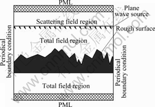
Fig. 1 Computation zones and boundary conditions used in wave reflection calculation from random roughness surface
Besides the mesh size, the time step size and the surface resolution, the other important FDTD simulation parameters for random rough surface scattering are the total surface length and total number of time steps. A longer surface length will ensure that precise surface statistics will be reflected in the simulations and better averages of the final results will be obtained. Sufficient time steps would be also required so that the steady state results are obtained. However, a long surface and a large number of time steps will significantly increase the computation time. A compromise between solution accuracy and computational time is necessary. At incident wavelength ��1=1.152 ��m and incident angle ��i=0o, the total surface length used in the simulation is 3 000��1 and the surface resolution is equal to the mesh size. For surface C, at ��1=1.152 ��m, the results are the average of two 3 000��1 surfaces to reduce the oscillations on the BRDF curves. The time step is ?t=0.5[(c/?x)2+ (c/?y)2]-1/2, where ?x=��/20, ?y=0.05 ��m. ?t is adjusted so that T* is an integer multiple of it. At this wavelength and incident angle, time steps are 15 000 for surface C.
At ��i=0�� and ��2=3.392 ��m, the total surface length used is 6 000��1. The same time steps are used in the ��1=1.152 ��m calculations. At ��i=30��, the results of surface C are shown here at wavelength ��1=1.152 ��m, and the surface length of 3 120��1 and 18 000 time steps are used; at ��2=3.392 ��m, the surface length of 6 360��1 and 18 000 time steps are used. At ��i=70��, the results of surface C are also shown here. For both wavelengths ��1 and ��2, the total surface length used in the simulation is 6 768��1 and time steps are 45 000. All the calculations are carried out on a 48-node cluster. A typical run would use 30 compute nodes and take computational time from 20 to 48 h.
Another problem that may arise due to insufficient surface length is the near-to-far-field (NTFF) transformation to obtain the reflectivity property [10, 13]. To demonstrate this problem, reflection of incident light at ��i=70o from surface C is calculated with NTFF transformation to obtain the BRDF. A flat surface reflection toward the specular direction of ��s=70o is shown in Fig. 2(a), which also uses NTFF transformation to obtain far field intensity. The Fraunhofer diffraction pattern is clearly shown near ��s=70o. Likewise, the BRDF of the rough surface C reveals the same diffraction for both TE and TM modes (Fig. 2(b)). The reflection of light incident at a large angle is then obtained by using three times the surface length in the NTFF transformation to mitigate the diffraction.
The BRDF of two different wavelengths at ��i=30�� are shown in Fig. 3. Overall, at a moderate incident angle, the FDTD simulation results are in good agreement with the measured data. However, as expected, the correlation is better at large wavelength (3.392 ��m) than that at small wavelength (1.152 ��m). At small wavelength, if the longer total surface length is used, the FDTD solution oscillations near the specular reflection direction would reduce. However, this seems to be redundant at this point. Since the ��/�� is smaller at a large wavelength, the specular or coherent component is stronger at ��=3.392 ��m.
Figure 4 depicts the TE and TM mode BRDF of two incident wavelengths at ��i=30��. At smaller wavelength of 1.152 ��m, there is little difference between the two modes. On the other hand, at 3.392 ��m, the TM mode BRDF is clearly smaller than that of TE mode for 0��<��s<50��, i.e., angles near the specular direction. The behavior is different from that at large incident angle.
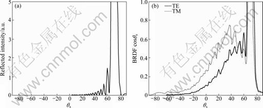
Fig. 2 Surface reflection at ��i=70o and with 3.392 ��m light source: (a) Flat gold surface with Fraunhofer diffraction; (b) Scattering from surface C (Fraunhofer diffraction pattern is apparent near specular reflection direction)
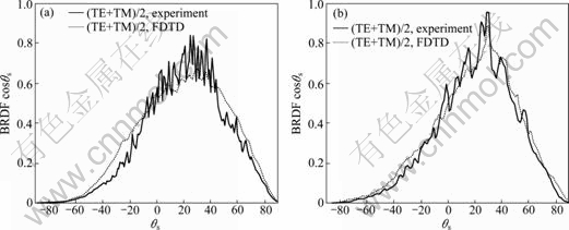
Fig. 3 Angular dependence of BRDF for ��i=30o and incident wavelength of 1.152 ��m (a) and 3.392 ��m (b)
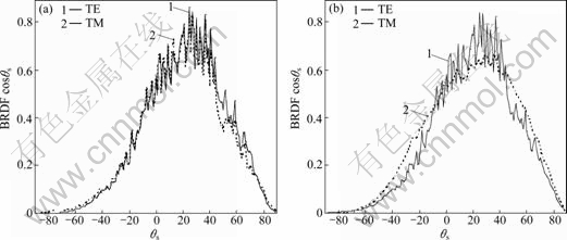
Fig. 4 Angular dependence of TE and TM mode BRDF at ��i=30�� based on FDTD calculations: (a) 1.152 ��m; (b) 3.392 ��m
At a very large incident angle of 70��, the TE and TM mode results of both FDTD and experiment are shown in Fig. 5. The agreement between the prediction and measurement at incident wavelength of 3.392 ��m is good, but somehow a larger difference at -10��<��s<40�� is seen at the incident wavelength of 1.152 ��m. In Fig. 5(a), for 0��<��s<40��, the experimental value for the TE mode is higher than the TM mode value. The FDTD curves confirm the difference but at a smaller level. On the other hand, at a incident wavelength of 3.392 ��m, both experimental and FDTD results show nearly the same higher TM mode than TE mode reflection. Furthermore, both results have nearly identical specular or coherent spike width at ��s=70��. The peak values of experimental TE and TM modes at the specular direction are not available from the work of KNOTTS and O��DONNELL [8]. However, the FDTD calculation shows that the TE mode value is more than twice of the TM mode value at the specular direction. Over a wide range of the non- specular scattering angles, TM mode values are larger than the TE mode values at 3.392 ��m and at a large incident angle, as shown in Fig. 5(b), which is drastically different from that at a smaller wavelength of 1.152 ��m (Fig. 5(a)) or at a smaller incident angle (Fig. 4(b)).
Clearly, the optical constant variation over the range from 1.152 to 3.392 ��m causes the switchover of TE and TM mode values at non-specular directions. The optical constants in Ref. [14] show two different values at several wavelengths but only the lower values, which are more consistent with the overall variation trend in the wavelength range, are used in the Drude model parameters of ��p and ![]() It is apparent that there is a sudden drop in ��p and sudden rise in
It is apparent that there is a sudden drop in ��p and sudden rise in ![]() near 1.24 ��m. The change in the Drude parameters causes the switchover of the TE and TM mode values in the non-specular directions. This is shown in the calculated BRDF variation over four different wavelengths in Fig. 6. Evidently, as the wavelength increases from 1.152 to 1.24 ��m, the TE and TM mode values are almost identical, except at and near the specular directions. Beyond 1.24 ��m, the TM mode values start to increase over the TE mode values at the non-specular directions. To understand the actual physical mechanism that causes the TE/TM mode switchover, for example, the surface plasmon polariton wave coupling [6], further study is needed.
near 1.24 ��m. The change in the Drude parameters causes the switchover of the TE and TM mode values in the non-specular directions. This is shown in the calculated BRDF variation over four different wavelengths in Fig. 6. Evidently, as the wavelength increases from 1.152 to 1.24 ��m, the TE and TM mode values are almost identical, except at and near the specular directions. Beyond 1.24 ��m, the TM mode values start to increase over the TE mode values at the non-specular directions. To understand the actual physical mechanism that causes the TE/TM mode switchover, for example, the surface plasmon polariton wave coupling [6], further study is needed.
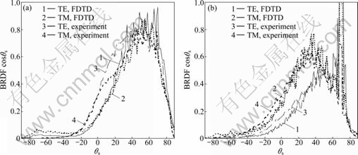
Fig. 5 Angular dependence of TE and TM mode BRDF at ��i=70�� and incident wavelength variation: (a) 1.152 ��m; (b) 3.392 ��m
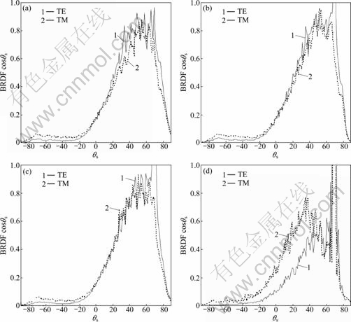
Fig. 6 Angular dependence of TE and TM mode BRDF at ��i=70�� and incident wavelength variation: (a) 1.152 ��m; (b) 1.24 ��m; (c) 1.442 ��m; (d) 3.395 ��m
4 Conclusions
1) The comparison with the accurate experimental data demonstrates that finite-difference time-domain method provides validated simulation capability to predict metallic surface radiative properties at various wavelength and surface roughness. The numerical solutions show good agreement with the reflectivity measured from a microscale random roughness Gaussian gold surface.
2) At a moderate incident angle of 30��, the correlation between the FDTD simulation and measured data is better at large wavelength (3.392 ��m) than that at smaller wavelength (1.152 ��m).
3) At a wavelength of 1.152 ��m, there is little difference between the TE and TM modes. But at 3.392��m, the TM mode BRDF is clearly smaller than that of TE mode for 0��<��s<50��.
4) At a very large incident angle of 70��, the correlation between the prediction and measurement at a 3.392 ��m incident wavelength is good, but somehow a larger difference in -10��<��s<40�� is seen at the incident wavelength of 1.152 ��m.
5) As wavelength increases from 1.152 to 1.24 ��m, the TE and TM mode values are almost identical. Beyond 1.24 ��m, the TM mode values start to increase over the TE mode values at the non-specular directions.
References
[1] BECKMANN P, SPIZZICHINO A. The scattering of electromagnetic waves from rough surfaces [M]. Norwood: Artech House, 1987: 170-180.
[2] DROLEN B L. Bidirectional reflectance and secularity of twelve spacecraft thermal control materials [J]. AIAA Journal of Thermophysics and Heat Transfer, 1992, 6(4): 672-679.
[3] HEBB J P, JENSEN K F, THOMAS J. The effect of surface roughness on the radiative properties of patterned silicon wafers [J]. IEEE Transactions on Semiconductor Manufacturing, 1998, 11(4): 607-614.
[4] TSANG L, KONG J A, DING K H. Scattering of electromagnetic waves [M]. New York: Wiley, 2000: 215-219.
[5] TANG K, KAWKA P A, BUCKIUS R O, Geometric optics applied to rough surfaces coated with an absorbing thin film [J]. AIAA Journal of Thermophysics and Heat Transfer, 1999, 13: 169-176.
[6] MCGURN A R, MARADUDIN A A, CELLI V. Localization effects in the scattering by light from a randomly rough grating [J]. Physics Review, 1985, B31(8): 4866-4871.
[7] MARADUDIN A A, MICHEL T, MCGURN A R, MENDEZ E R. Enhanced backscattering of light from a random grating [J]. Annals of Physics, 1990, 203: 255-307.
[8] KNOTTS M E, O��DONELL K A. Measurements of light scattering by a series of conducting surfaces with one-dimensional roughness [J]. Journal of the Optical Society of America A, 1994, 11(2): 697- 710.
[9] YEE K S. Numerical solution of initial boundary value problems involving Maxwell��s equations in isotropic media [J]. IEEE Transactions on Antennas and Propagation, 1966, 14(3): 302-307.
[10] BOHREN C F, HUFFMAN D R. Absorption and scattering of light by small particles [M]. New York: John Wiley & Sons, 1983: 233- 246.
[11] KUNZ K S, LUEBBRES R J. The finite difference time domain method for electromagnetics [M]. Boca Raton: CRC Press, 1993: 68-76.
[12] TAFLOVE A, HAGNESS S C. Computational electrodynamics: The finite-difference time-domain method [M]. 3rd Ed. Boston: Artech House, 2005: 110-116.
[13] ZHAO Y, WANG G C, LU T M. Characterization of amorphous and crystalline rough surface: Principles and applications [M]. San Diego: Academic Press, 2001: 237-354.
[14] PALIK E D. Handbook of optical constants of solids [M]. Orlando: Academic Press, 1985: 50-60.
(Edited by HE Yun-bin)
Foundation item: Project(N110204015) supported by the Fundamental Research Funds for the Central Universities
Received date: 2011-03-28; Accepted date: 2011-08-05
Corresponding author: WANG Ai-hua, PhD; Tel: +86-13624210542; E-mail: wangaihua1976@yahoo.com.cn
Abstract: The radiative properties of a gold surface with one-dimensional Gaussian random roughness distribution were obtained with the finite-difference time-domain (FDTD) method and the recursive convolution treatment of the Drude Model. The bi-directional reflection distribution function (BRDF) for both TM mode and TE mode were obtained and compared with the highly accurate experimental data from the earlier work. The incident wavelength varies from 1.152 ��m to 3.392 ��m and incident angle is at 30��-70��, respectively. The results show that, the predicted values and experimental results are in good agreement. The highly specular peak in the BRDF is reproduced in the numerical simulations, and the increase of the TM mode BRDF is found to be attributed to the effect of a variation in the optical constant at the incident wavelength period.
