

J. Cent. South Univ. (2021) 28: 1747-1764
DOI: https://doi.org/10.1007/s11771-021-4730-x

Rotation forest based on multimodal genetic algorithm
XU Zhe(�솴)1, 3, NI Wei-chen(��ά��)2, JI Yue-hui(���»�)1, 3
1. School of Electrical and Electronic Engineering, Tianjin University of Technology, Tianjin 300384, China;
2. Academic Affairs Office, Tianjin University of Technology, Tianjin 300384, China;
3. Tianjin Key Laboratory for Control Theory & Applications in Complicated Industry Systems,Tianjin 300384, China
 Central South University Press and Springer-Verlag GmbH Germany, part of Springer Nature 2021
Abstract:
In machine learning, randomness is a crucial factor in the success of ensemble learning, and it can be injected into tree-based ensembles by rotating the feature space. However, it is a common practice to rotate the feature space randomly. Thus, a large number of trees are required to ensure the performance of the ensemble model. This random rotation method is theoretically feasible, but it requires massive computing resources, potentially restricting its applications. A multimodal genetic algorithm based rotation forest (MGARF) algorithm is proposed in this paper to solve this problem. It is a tree-based ensemble learning algorithm for classification, taking advantage of the characteristic of trees to inject randomness by feature rotation. However, this algorithm attempts to select a subset of more diverse and accurate base learners using the multimodal optimization method. The classification accuracy of the proposed MGARF algorithm was evaluated by comparing it with the original random forest and random rotation ensemble methods on 23 UCI classification datasets. Experimental results show that the MGARF method outperforms the other methods, and the number of base learners in MGARF models is much fewer.
Key words:
ensemble learning; decision tree; multimodal optimization; genetic algorithm��
Cite this article as:
XU Zhe, NI Wei-chen, JI Yue-hui. Rotation forest based on multimodal genetic algorithm [J]. Journal of Central South University, 2021, 28(6): 1747-1764.
DOI:https://dx.doi.org/https://doi.org/10.1007/s11771-021-4730-x1 Introduction
Ensemble learning is one of the main research areas of machine learning [1-3], and it is widely used in many fields such as fault detection and diagnosis [4-6], image recognition [7, 8], face recognition [9, 10], and data stream analysis [11, 12]. The main feature that the ensemble model is more accurate than the single model has been proved by TUMER et al [13] and BROWN et al [14]. DIETTERICH [2] explained the reason for the enhanced performance of the ensemble model from the perspective that the ensemble model can find the optimal hypothesis in the hypothesis space.
Multiple types of decision trees are commonly used as base models of ensembles for these algorithms are simple, efficient, and fast [15-18]. Besides, the structural complexity of decision trees can be easily and accurately controlled by tuning the depth parameter. Furthermore, the decision trees are of high variance due to their susceptibility to the variation in the training data. This striking feature facilitates the generation of diversity among base�� models. Moreover, decision trees can work directly with the dataset consisting of continuous and categorical variables, and even the variables with missing values.
There are many tree-based ensemble approaches. The Random Forest (RF) is one of the most famous tree-based ensemble methods [19, 20]. It utilizes the feature selection and random subspace method for injecting diversity into ensembles. The Rotation Forest is another tree-based ensemble method [21]. It selects feature subsets from the feature space, similar to RF, but the chosen feature subsets will be rotated to inject randomness. The Random Rotation Ensemble (RRE) method was proposed by BLASER et al [22]. It achieves the random injection using the characteristic of the decision tree to be very sensitive to the rotation of the training samples. The advantage of this method is that the randomness injection is achieved by random sample rotation, rather than random sample selection, such as Random Forest, Rotation Forest, and Bagging algorithms [23]. This advantage is apparent when the amount of data is small because all but not part of the data can be used for modelling.
Since all the base models of the above algorithms are randomly generated, each of these ensemble models would require an infinite number of the random base models, theoretically, to ensure the convergence. In practice, the number of random base models is a problem-dependent parameter, which is and should be of considerable value in most cases.
In addition to the number of base models, the diversity and accuracy of base learners are also crucial to the success of the ensemble model [24]. However, the two factors are contradictory [25]. When the diversity among base learners increases, the accuracy of the base learners will decrease, and vice versa. So, it is essential and a challenge to balance between the two critical factors in ensemble modelling.
There are various selective ensemble algorithms proposed to find the optimal balance between the accuracy and the diversity of base learners to improve the accuracy of ensembles. GASEN is a selective ensemble method, which can obtain a good generalization result [26]. In this method, instead of all models, a set of models are selected as base models in terms of weight coefficients optimized by genetic algorithm to form an ensemble model. Similar to the GASEN method, optimized weight coefficients are used to choose base learners in the WAD method proposed by ZENG et al [27]. The optimization goal in WAD is not just the accuracy of the ensemble model, but the target combined with accuracy and diversity.
Both of the above methods have one feature in common: the base models are selected from all candidate modes according to the optimal solution of genetic algorithm (GA). The composition of candidate models is also an important issue, which is missing from the above methods. If the candidate models are randomly generated, it is necessary to have a large number of candidate models as a guarantee of maintaining an appropriate balance between the diversity and accuracy of base models. In fact, if the number of candidate models is too large in GA, it will increase the number of decision variables, increase the search space, and reduce the search speed.
Multi-objective optimization is used in Ref. [28] to select base learners, which takes the model accuracy and diversity as two optimization goals. In this method, the diversity among base models selected by the multi-objective algorithm can not be guaranteed because the base models are selected according to a one-to-many comparison approach. That is, the outputs of each model are compared with the average outputs of all the candidate models. Moreover, the models with high diversity and low accuracy are also selected as base models. However, these selected base models may not contribute much to improving the accuracy of the ensemble model.
To avoid the shortcomings of the previous methods and improve the accuracy of decision tree based ensemble algorithm, a multimodal genetic algorithm based rotation forest is proposed for classification problems in this paper, called multimodal genetic algorithm based Rotation Forest (MGARF). The proposed method aims at building a selective tree-based ensemble with diverse and reasonably accurate base models.
The main improvement consists of using the multimodal optimization algorithm as the tree selection method. The optimization result of multimodal optimization is a solution set composed of multiple local and global optima individuals. Furthermore, the diversity among individuals in the solution set can be guaranteed by using the diversity preservation strategy that is an inherent function of the multimodal optimization. Also, in MGARF, base models are determined by the optimization solutions, and there is a one-to-one correspondence between them. Thus, the choice of the multimodal optimization algorithm appears to be reasonable.
In comparison with the existing selective ensemble methods, candidate models of MGARF are dynamically generated under the directions of evolutionary operations, which are superior to the randomly pre-generated models. Moreover, the number of these candidate models is not limited to a fixed number, and the number of candidate models does not affect the search space of the optimization algorithm.
Multimodal optimization is a combination method of a global metaheuristic optimization called the core algorithm, and a niching technique used as a preserve preservation method to allow the optimization results to converge to multiple local and global optima solutions.
Several metaheuristic optimization methods have been used as the core algorithm, such as GA, differential evolution (DE), and particle swarm optimization (PSO). Both the GA and DE metaheuristic optimization methods belong to the evolutionary algorithm inspired by the biological view of organismal evolution in nature.
The GA algorithm was originally used as the core algorithm of multimodal optimization, and many niching methods were proposed in combination with GA to provide diverse niches, such as clearing [29], crowding [30], fitness sharing [31], and species conservation methods [32].
The sharing method is the first attempt to solve multimodal optimization using the niching method. This method shares similarity values measured between individuals within the same subgroup. The crowding method simulates competition among similar individuals for limited resources. In this method, a parent can be replaced by its similar offspring with better fitness. The species conservation method is proposed based on the notion of species, into which the population is divided according to their similarity. Within each species, there is a species seed, a dominating individual, and will be passed on to the next generation to be conserved. This niching method only introduces one parameter, species distance, as the upper limit on the distance within a species. This feature facilitates parameter tuning and makes it easier to obtain optimal solutions. Thus, this method is used as the multimodal optimization in our proposed method. Similarity evaluation is an essential part of the above niching methods, and it can be measured by the Hamming or Euclidean distance metric for binary-coded variables or real variables, respectively.
Multimodal optimization methods with DE and PSO as core algorithms have been a growing area of recent research, such as the sharing DE [33], crowding DE [33], species-based DE [34], BMDE [35], ANDE [36], and PSO based EDHC [37]. Many research works have recently been focusing on the adaptive capability of multimodal optimization. DSDE [38] and SDLCSDE [39] methods adaptively select an algorithm parameter. An adaptive mutation strategy is used in AGDE [40]. CLPSO-LS [41] was proposed to determine the adaptive starting criterion for the local search method. Other new multimodal optimization methods have surfaced recently, including the chaos optimization-based NCOA [42] and RCSA Cuckoo Search [43] that uses the reinforced cuckoo search algorithm.
The main contribution of this paper is the multimodal optimization based selective ensemble scheme, which may prove to be useful in practical applications of ensemble learning. Furthermore, a specifically designed chromosome encoding and decoding method based on householder reflection is proposed and proven to solve GA based multimodal optimization, which is the basis of this proposed scheme.
The remainder of this paper is organized as follows. Section 2 shows an overview of our framework and implementation details of the MGARF algorithm. Then, experimental methods and results are presented in Section 3, and Section 4 concludes the work.
2 Modelling methods
The schematic diagram of the proposed MGARF algorithm is shown in Figure 1. For simplicity, only the process flow in the last generation of the GA-based multimodal optimization is illustrated in this figure, for the processes in other generations that are omitted in this figure are similar to those in the last generation. The genetic operations and the operations of multimodal optimization that are omitted will be presented later in Section 2.2.
In this algorithm, the phenotypes to be optimized are the rotation angles of the original data, and each decision tree is constructed with its corresponding rotated data. The optimal set can be obtained according to the accuracy and similarity measurements of their corresponding decision trees [44]. The rotation forest is composed of all base learners whose corresponding rotation angles are in the optimal set.
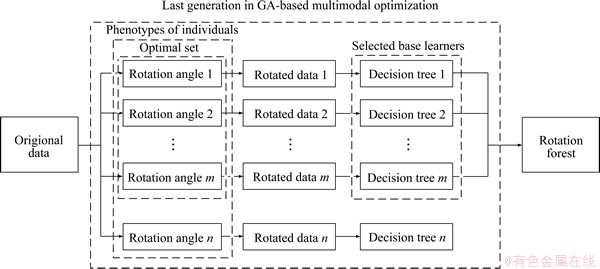
Figure 1 Schematic diagram of optimization process in last generation
2.1 Characteristic of decision tree
A graphic example is used to illustrate the unique character of the decision tree. The classification results showed in Figure 2 are obtained from two different decision tree models, which are built using the same decision tree modelling method. The samples in Figure 2(b) are obtained by rotating the samples 15�� clockwise in Figure 2(a). In Figure 2(a), two types of samples are separated by one decision boundary. However, there are two decision boundaries in Figure 2(b), and the data are not correctly separated. That is, although the ensemble model became complicated, the classification accuracy is decreased.
This example intuitively demonstrates that the decision tree is sensitive to the rotation of samples because the decision boundaries of the tree can only be parallel to the coordinate axes. This example also shows that this character can be used to inject randomness into the decision tree based ensemble model, and the diversity between trees will increase as a result.
2.2 Multimodal optimization method
Combined with niching techniques, the genetic algorithm can be used to solve multimodal optimization problems. Our proposed method combines species conservation strategy, one of the niching techniques, with GA as a multimodal optimization method to select optimal rotation angles. Similar to the multi-objective optimization algorithm, this combined algorithm can also obtain multiple solutions. However, unlike the multi-objective optimization algorithm, there is only one single optimization objective in the GA-based multimodal optimization method.
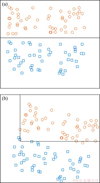
Figure 2 (a) Decision boundary before data rotation;(b) Decision boundaries after data rotation
2.2.1 Seeds identification method
Seeds are some representative individuals in a population, and the identification of seeds is the basis for the optimization process. The seeds identification method is presented in Algorithm 1.
Algorithm 1 Procedure of seeds identification

The fitness value of the individual pi is calculated using Eq. (1) that is the misclassification rate corresponding to pi:
 (1)
(1)
where I(��) is the indicator function; T(xn, pi) is the classification result of the base learner T at xn with the rotation angle corresponding to pi; yn is the actual value for observation xn; and N is the number of data.
Individuals with better fitness are preferentially selected as seeds in the seeds set S{sj | j=1, ��, Ns}, where Ns is the number of seeds. As the individuals in the optimization represent data rotation angles, ����(a, b)=|��a-��b| is used to evaluate the difference between two individuals, where ��a and ��b are rotation angles corresponding to individuals a and b. A smaller angle difference indicates higher individual similarity. The computed difference between any two seeds is not allowed to be less than the similarity threshold ��, which ensures the diversity among seeds.
The search for a better value of �� for each specific dataset is time-consuming. Instead, the following two rules are applied to adjust �� adaptively in every optimization generation.
Rule 1: if Ns<��Np, ��=��-��
Rule 2: if Ns>��Np, ��=��+��
where �ǡ�(0,1] is a parameter that needs to be set in advance; and �� is an increment for adjustment. It can be seen that Ns is inversely proportional to ��.
2.2.2 Species identification
In evolutionary algorithms, a species is a sub-population in which individuals have high similarity with each other, but the similarity among individuals from different species is low. The species identification method is to split the entire population into disjoint subpopulations Ej (j=0, ��, l). Each subpopulation is a distinct species. The species Ej (j=1, ��, l) are within the area centered at their respective seeds sj (j=0, ��, l) with a radius of ��/2. The species E0 contains all individuals not included in species Ej (j=1, ��, l). The pseudo-code description of this procedure is presented in Algorithm 2.
Algorithm 2 Procedure of species identification method

The similarity values between every two individuals are evaluated in a population to identify each species. If the similarity value between two individuals is less than ��, they belong to the same species; otherwise, they belong to different species.
2.2.3 Species conservation method
Seeds are the best-fit individuals in their species, and there is a certain difference between each seed, so all the seeds are candidates for the optimal solution. The species conversation method is used to transfer seeds to the following generations to avoid the destruction of good genes in seeds due to selection, crossover, and mutation operations. The species conservation procedure is shown in Algorithm 3.
Algorithm 3 Procedure of conserving species
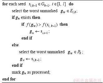
In this procedure, si,k-1 is the i-th seed in the k-1 generation, and Gk-1 is the seed set that contains all the seeds in the k-1 generation. Ei,k is the i-th species in the k-th generation, and the seed si,k-1��Ei,k. gw is the individual in the k-th generation to be replaced by the seed in the k-1 generation.
2.2.4 Overall flow of MGARF algorithm
The procedure of the proposed method is shown in Algorithm 4.
Algorithm 4 Procedure of MGARF algorithm
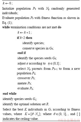
In addition to genetic operations such as crossover and mutation, seeds identification, species identification, species conversation, and optimal solution identification are also included in this algorithm. The optimal solution set is composed of seeds, but not all the seeds are included. Instead, only a part of seeds with better fitness values is selected to form the optimal solution set in optimal solution identification. According to the fitness values, the top K seeds are chosen as the solution set. K is the value rounded up to the nearest integer of �ȡ�Ns,�ȡ�(0,1] is a parameter to be determined; Ns is the number of individuals in Gs.
2.2.5 Analysis of computational complexity of MGARF algorithm
The complexity of the proposed algorithm is mainly determined by the fitness evaluation and the species conserving technique based multimodal operations.
The fitness evaluation is an essential part of the genetic algorithm, whose complexity is O(Np��D), where Np is the population size; and D is the number of generation iterations. The worst case is Np��Dmax, where Dmax is the maximum number of generation iterations allowed in the termination condition.
The multimodal operations include seeds identification, adjustment of the parameter ��, species conservation, and optimal solution identification, among which seeds identification and species conservation are more computationally intensive. The main computational burden of these two procedures comes from the evaluation of the distance between two individuals. Thus, the times of distance measurements to be carried out are chosen to present the computational complexity in multimodal operations [32].
The lower and upper limits for execution times of distance calculation in seeds identification (Os) and seed conservation (Oc) are shown in Eqs. (2) and (3).
 (2)
(2)
 (3)
(3)
where Ns is the number of species to be identified for each generation, and it is determined by ��; and �� is adjusted automatically according to the parameter ��. It means that N��, the upper bound on Ns, can be given based on ��.
The upper bound on Oc is also linear with N��. The total complexity Osc, Osc=Os+Oc, is presented in Eq. (4):
 (4)
(4)
When the value of N�� increases to Np, the upper bound of the complexity of Osc is  which is the worst case. Such a high computational complexity will not be reached under normal circumstances, and the normal computational complexity should be O(Np).
2.3 Encoding and decoding method
Householder reflection is used to rotate the samples in multi-dimensional space [45]. This method is a linear transformation using the transformation matrix H that is calculated as:
 (5)
(5)
where ||��|| is L2-norm; w is an n-dimensional unit vector; w* is the conjugate transpose of the vector w; I��Rn��n is an identity matrix; and H��Cn��n is a unitary matrix. The vector v��Cn and its image vector Hv are mirror-symmetric about the hyperplane with normal vector w, as in Figure 3.
The angle between v and Hv can be regarded as the rotation angle from v to Hv, and the magnitude of the rotation angle can be considered as determined by w.
Thus, the normal vector w is encoded into real value chromosomes in the GA-based optimization for searching among all the possible rotation angles. Specifically, consider a given data pair (x, y). There are q numeric attributes in the p-dimensional predictor x, and y is a categorical variable. In the rotation process of variable x, only the q numeric features are rotated, as the rotation of categorical features is ineffective for decision tree modelling. According to the q numeric attributes in x, each individual is encoded as a q-1 dimensional vector c={ci|i=1, ��, q-1}��Rq-1, and ci��[-1, 1], i=1, ��, q-1. In the decoding process, the vector c is used to calculate the q-dimensional vector d:
 (6)
(6)
where dq��[0, 1]. It is possible to obtain the normal vector w=d/||d|| from its corresponding chromosome using this encoding and decoding method.
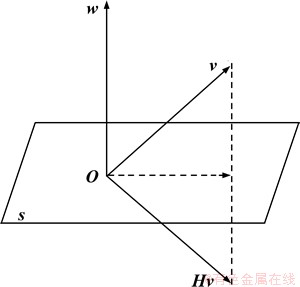
Figure 3 Vector v and Hv are mirror-symmetric about hyperplane s
Theorem 1: This encoding and decoding method enables a one-to-one mapping between the chromosome and the normal vector.
Proof: Suppose there are two different encoding vectors b and a corresponding to the same q-dimensional normal vector w. Let r and s be the decoded vectors of b and a, respectively. Due to Eq. (6), we have bi=ri and ai=si (i=1, ��, q-1). Because w is the normalized vector of r and s, it implies r=ks, and b=ka, where k is a real number and 
Since  and
and  we have:
 (7)
(7)
Combining bj=kaj, j��[1, q-1], we have that
 (8)
(8)
we can get
 (9)
(9)
k=1 can be obtained from Eq. (9), that is r=s and b=a. It can be concluded that the uniqueness of this chromosome encoding and decoding method can be guaranteed.
Lemma 1: The normalized q-dimensional normal vectors obtained through this encoding and decoding method can represent all the q-dimensional unit vectors with the q-th dimension within the range [0, 1].
Proof: Given the encoding vector b with q-1 dimensions and its decoded vector r with q dimensions, all the elements in b and the first q-1 elements in r are in the range of [-1, 1], and the range of the q-th element rq in r is [0, 1] as described above. For bi, bj��b (i, j��[1, q-1], and i��j), the ratio of bi to bj is:
 (10)
(10)
where  is the average of all the elements in b. and the relative value of rq andis:

 (11)
(11)
Since  , the range of rq/is:
 (12)
(12)
Combine Eq. (10) with Eq. (12), and we get rq/bi��(-��, ��), i��[1, q-1], which means that rs/rt��(-��, ��) (s, t��[1, q] and s��t), as bi=ri, i��[1, q-1]. It indicates that the ratios of any two elements in r range from -�� to ��. If the range of rq is the same as those of other elements in r, the vector w obtained by normalizing r can represent any q-dimensional unit vectors. The actual range of rq is [0, 1]. Therefore, only these unit vectors corresponding to wq��[0, 1] can be represented through this encoding and decoding method.
Theorem 2: With this chromosome encoding and decoding scheme, all possible rotation angles can be represented.
Proof: The proof of Theorem 2 relies on Lemma 1. Since ww*=(-w)(-w)* and the relation between w and H from Eq. (5), we can get that both w and -w correspond to the same matrix H that determines the rotation angle. It means the rotation angle corresponds to the decoded vector [r1, r2, ��, rq-1, -rq] can also be obtained from [-r1, -r2, ��, -rq-1, rq]. Thus, the value range of rq only needs to be [0, 1] instead of [-1, 1]. And because of Lemma 1, this encoding and decoding scheme does not reduce the range of rotation angles but avoids the repetition of the rotation angles.
3 Experiments and results
Random Forest and Random Rotation Ensemble methods were used for comparison to evaluate the performance of the proposed MGARF method. Many applications suggest that RF is a state of art ensemble learning algorithm [46]. Each decision tree in the RRE model is built after a random rotation of the entire training data. Unlike the proposed MGARF method, RF and RRE combine all the trained decision trees as base learners without selection. These methods are all ensemble learning techniques, and the base learners within these methods were constructed using classification and regression trees (CART) [47, 48]. In other words, the focus of the following experiments is on comparing the performance of CART based ensemble algorithms.
3.1 Datasets and data preprocessing
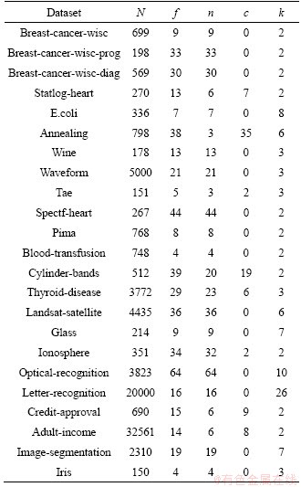
The experiments are based on twenty-three datasets obtained from the UCI repository [49]. The details of the datasets are shown in Table 1, where N is number of observations; f is number of features; n is number of numeric features; c is number of categorical features; k is number of classes.
Each dataset was randomly split into a training set, a testing set, and a validation set. The validation set consisted of 20% of the original data, 70% of the remaining samples in the original dataset were used as the training set, and the rest of the data were used as the testing set.
For the MGARF method, base learners were built on the set of training data; fitness values in the optimization process were calculated using the testing set and the final ensemble models were evaluated using the validation set. For RF and RRE methods, base learners were also built on the training set, and the validation set was used to test the ensemble models.
Table 1 Datasets for experiments
For numeric features, a basic scaling method was used in the data preprocessing step. This scaling method scales the numeric value xi,j, the i-th dimension of the j-th sample, according to the maximum and minimum values of the i-th dimension to range between 0 to 1. The scaled value  of xi,j can be calculated as:
 (13)
(13)
The maximum and minimum values are all in-sample values. If a sample exceeds the in-sample range, it will be set to 0 or 1, depending on which value is closer to it. Then the following procedure was performed to distinguish between numeric and categorical variables and to handle missing data.
1) Any column with non-numeric values or with the number of distinct numeric values less than 10 was treated as a categorical variable, and the other columns were treated as numerical variables.
2) For categorical missing data, a new category was created. The missing numerical data were set as the median of its column values.
3) Every categorical variable with C categories was transformed into dummy variables with C-1 0 or 1 values [50].
3.2 Stopping criteria and parameters
The following two stopping conditions were employed for the multimodal optimization procedure of the MGARF algorithm.
One is that |fa(k)-fa(k-1)|<>l holds for n consecutive generations and k>Gmin; and the another is k >Gmax.
The first condition evaluates whether the possibility of achieving a considerable improvement in the subsequent generations is low. It is a phenotypical termination rule, and the average fitness fa(��) is used, where fa(k) is the average fitness of the current generation (k-th generation). The parameter Sl is a threshold; Gmin represents the minimum number of generation iterations allowed; and Gmax is the upper limit on the number of generations.
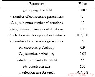
For all datasets, the main parameters for MGARF were set to the values listed in Table 2.
The parameter �� and �� are two important selection rates affecting the number of base learners in MGARF. In the following experiments, the �� and �� were set to 0.7 in MGARF-0.7 and 0.8 in MGARF-0.8. The numbers of base models in MGARF-0.7 and MGARF-0.8 are about 49% and 64% of the population size, respectively. Thus, models built with these two values of �� and �� can demonstrate the performance of MGARF models of moderate complexity.
Table 2 Main parameters for MGARF
In RF, the number of feature variables to select at random for each decision split is set to the square root of the total number of variables. A portion of samples was randomly selected with replacement for each bootstrap replica in RF. The size of each replica is 0.9Nt, where Nt is the total number of samples in the training set. There is no additional parameter in RRE.
The classification and regression trees (CART) base learners were grown without pruning. All experiments were repeated ten times.
3.3 Method and comparison
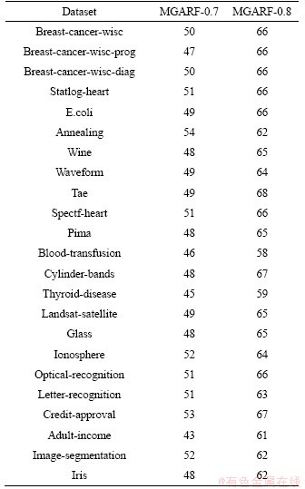
The exact average numbers of decision trees in models of MGARF-0.7 and MGARF-0.8 are listed in Table 3. The average numbers of trees in MGARF-0.7 and MGARF-0.8 are 49 and 64, respectively.
To compare the three algorithms with the same number of base learners, the numbers of trees in RF-64 and RRE-64 models were the same as that in the MGARF-0.8 model corresponding to the same dataset. The number 64 represents the overall average number of base learners in MGARF-0.8 models. In the hope of achieving better accuracy of RF and RRE models, the numbers of trees within MGARF-0.7 models were not chosen as the reference values, as their base learners are fewer than those within MGARF-0.8 models. RF-200, RF-500, RRE-200, and RRE-500 models were built to compare with ensemble models with multiple base learners. The numbers 200 and 500 indicate the numbers of trees.
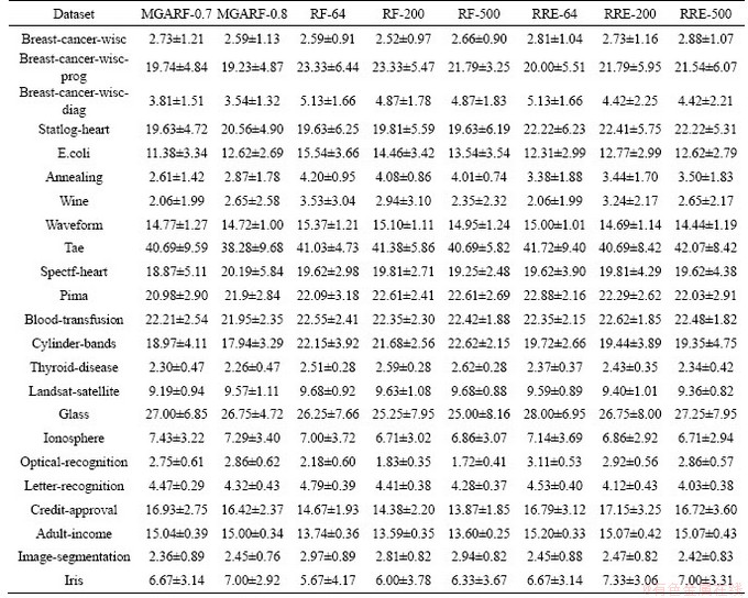
The mean and standard deviation of the classification errors on benchmark datasets are listed in Table 4.
Table 5 presents the rankings of different methods, according to Table 4. The values ranging from 1 to 8 in each row are the rankings of the eight different models for a dataset. The smaller the ranking, the better the classification accuracy. If both the means and standard deviations of classification errors of different models in the same row were the same, then the rankings of these models were set to the average value of their original rankings.
Table 3 Average numbers of decision trees in MGARF models
Average rankings are listed in the last row of Table 5, representing the overall performance of different methods on all the datasets. Although the average rankings of MGARF methods were smaller than the others, the classification accuracy of MGARF models did not always outperform the others on every dataset.
Friedman��s test was used to make sure these methods are different significantly [51]. According to Table 5, The Chi-Squared value of Friedman��s test is 19.67, and the p-value is 0.0063 at the confidence of 95%. Thus, the null hypothesis can be rejected. Therefore, it means that the impact of these methods is different significantly.
Among three RF methods, RF-500 performed more accurately than the other two methods, RF-64 and RF-200, on 12 datasets, accounting for only 52% of all the 23 datasets. Similarly, among the three RRE methods, RRE-500 did not achieve the highest accuracy on all datasets. This result suggests that high uncertainty is introduced into RF and RRE models through the randomly generated base models. A large number of base models cannot guarantee the accuracy of the ensemble, for the RF will not converge until the number of base models approaches infinity. It shows that the selection of random base models in the ensembles is necessary to obtain more accurate ensemble models. Furthermore, the effectiveness of the base model selection scheme has been confirmed in the experiments. The results of both MGARF methods, MGARF-0.7 and MGARF-0.8, are better than those of the RF and RRE models in terms of the average ranking in Table 5.
Table 4 Mean and standard deviation of classification errors (%)
Tukey Kramer multiple comparison [52] was used to determine the significant differences between each method in Table 5 accurately, and the comparison results are shown in Figure 4.
In Figure 4, the x-axis and y-axis represent rankings and modelling methods, respectively. The average rankings of these methods are shown as circles. If the two methods are significantly different, the intervals, the line extending out from the circles, are not overlapped. Otherwise, the two methods are not significantly different. It can be seen that just MGARF-0.7 is significantly different from RF-64 and RRE-64. In general, the two MGARF methods with different parameters are not significantly different from all the other methods.
For RF and RRE models, the average rankings were improved with increasing the number of base learners, and the best rankings of the two ensemble methods were achieved by RF-500 and RRE-500 separately. It is consistent with the ensemble learning principle that the accuracy of the ensemble model tends to improve as the number of base learners increases. However, there are fewer base models in MGARF-0.7 than in MGARF-0.8, but the average ranking of MGARF-0.7 is better than that of MGARF-0.8. This observation is related to the selective integration feature of the MGARF method, which maintains diversity among base learners throughout the whole optimization process.
Table 5 Rankings of different methods correspond to Table 4
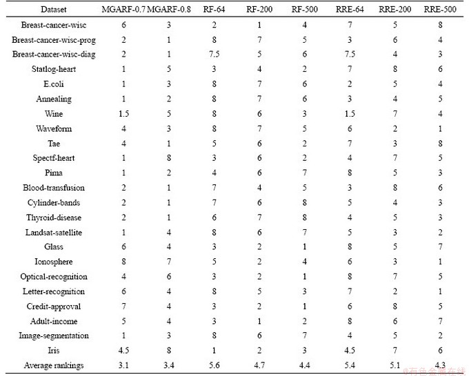
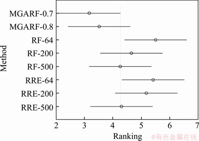
Figure 4 Multiple comparison of different modeling methods
The three algorithms, MGARF, RF, and RRE, were compared using the best case of each algorithm, and the rankings are listed in Table 6.
The p-value of the Friedman��s test of this comparison is 0.0125 at the confidence of 95%, and the multiple comparison with a 95% confidence interval is performed, and the results are shown in Figure 5 and Table 7. The intervals of MGARF do not overlap with the others in Figure 5. In the first two rows of Table 7, the value 0 does not fall within the upper and lower limits, and the p-values are small, 0.0199, and 0.0161, which indicates that the MGARF is significantly different from RF and RRE. Furthermore, the average ranking of MGARF was the smallest, and the numbers of base learners within MGARF models were no more than those within RF and RRE models. The MGARF algorithm has apparent advantages over RE and RRE algorithms in terms of classification accuracy and model complexity.
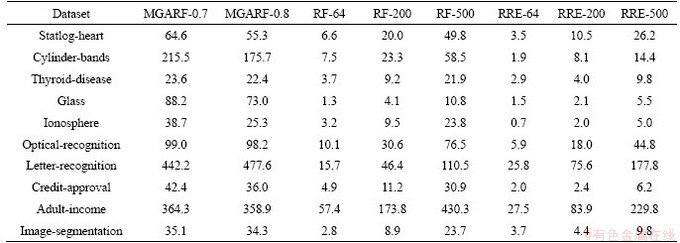
The computing speed tests were carried out using MATLAB 2018b on a Windows-based machine with 4 cores 3.2 GHz Intel I5 CPU, 32GB memory. Each method was run ten times on each dataset listed in Table 8. The average computing time is presented in this table.
Table 6 Rankings of best case of each algorithm
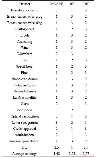
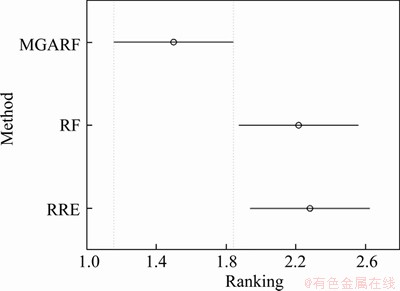
Figure 5 Multiple comparison of MGARF, RF and RRE algorithms
As different implementation codes were used, the execution time of RF and RRE methods are different for the same number of base models in the same dataset.
3.4 Effect of parameters
The parameter �� is the ratio of the number of optimal individuals to the number of seeds, and �� is the selection rate for optimal individuals. They are two critical parameters in the MGARF algorithm affecting both model accuracy and the number of base learners. Both parameters have a value range of [0, 1]. The experiments of the effect of parameters �� and �� in MGARF were carried out with the IRIS dataset. The parameters �� and �� ranged from [0.1 1] in intervals of 0.1. We ran the experiments ten times for each combination of both parameters, and the mean classification errors of these experiments are listed in Table 9.
Table 7 Results of Tukey Kramer multiple comparison
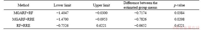
Table 8 Average computing time for modeling (s)
Both parameters are proportional to the number of base learners. However, as the number of base learners increases, the accuracy of the ensemble model may not necessarily be improved. The best mean classification accuracy error was 4.00%, with only two base models when ��=0.1 and ��=0.2. It is the most accurate classification result compared to all methods for the iris dataset in Table 4.
Since the selective property of the MGARF algorithm, this method did not produce large errors in this dataset, even with only one base model (��=0.1 and ��=0.1). The mean error of the entire table is 6.20%. Even if the search interval is increased to 0.3 or 0.5, the worst case (8.00%) can be avoided, and relatively high accurate ensembles can be obtained. Therefore, instead of using heuristic optimization algorithms to optimize the two parameters, the above simple grid search method can obtain a suitable result through multiply tests.
3.5 Diversity-error analysis
Kappa-error diagram [53] is commonly used to analyze the diversity-accuracy behavior of ensemble models, which is an effective way to explain why the ensemble models perform differently. In the Kappa-error diagram, the x-coordinate is the kappa value (pairwise diversity), and the y coordinate is the average individual error. In this paper, the average individual error is the average classification error calculated from the classification errors of two base learners.
The Cohen��s kappa (or kappa statistic) �� is a similarity coefficient [54, 55], which can be used to evaluate the similarities between base learners by using their classification results. There are several evaluation methods of model similarity, and the kappa coefficient is more accurate than others, especially when the sample imbalance occurs because it considers the agreement occurring by chance.
Two base learners determine the value of �� ranging from -1 to 1. A high value of �� indicates the low similarity of the two base learners. ��=1 means that the classification results of two base learners are in complete agreement, indicating that the two base learners are identical. When ��=0, the two classifiers are agreed by chance. ��<0 indicates that there is a specific disagreement between the two base learners.
There is a situation to be aware of when calculating ��. If all the outputs of the two models are the same, and the classification result of a model only contains one category. In other words, all the predicted values in the classification results of two base learners are the same. The divide-by-zero error will occur. In this case, �� can be set to 1 because of the similarity of the outputs of the two models.
Three representative datasets (Image-segmentation, Thyroid-disease, and E.coli) were selected to compare the ensemble models built by three modelling approaches (RRE, RF, and MGARF). The plots are shown in Figure 7.
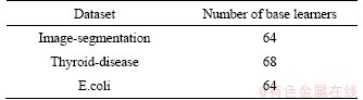
The parameters �� and �� of MGARF were both set to 0.8. For each dataset, three models were built with the same number of base learners, and the number was determined by the MGARF model. The statistical characteristics represented by a point in the figure are of two base learners. Thus, there will be n(n-1)/2 points representing all the pairwise characteristics in an ensemble model with n base learners. The numbers of base learners are listed in Table 10.
Table 9 Mean classification errors of 10 experiments on the iris dataset modeled by MGARF (%)
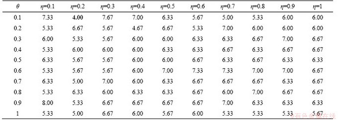
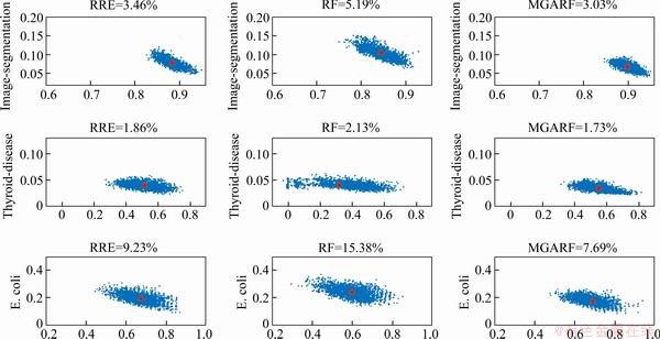
Figure 6 Kappa-error diagrams
Table 10 Number of base learners
The triangle marks the centroid of kappa-error points in each plot, and the classification error rates are listed at the top of plots. Unlike previous experiments, the classification error and number of base learners are of one ensemble model, not the average values of multiple models.
All plots displayed in a row correspond to the same dataset, and the scales of �� (x-axis) and error (y-axis) of these plots are the same. It is evident from the plots that the diversity and accuracy in ensemble models are indeed contradictory, and as one increases, the other decreases, and vice versa.
The MGARF method has the lowest model diversity for each dataset, while it has the highest pairwise model accuracy, giving it the lowest total classification error. This performance is due to the selective feature of the MGARF method, which removes some of the less accurate base models, and the diversity among the preserved base models is reduced. The RF method has the widest range of kappa values compared to RRE and MGARF, and its average kappa value is also the lowest, but it has a high level of error, resulting in a high overall classification error. The RRE method is neither as diverse as RF nor as accurate as MGARF, and its overall classification error is between RF and MGARF.
It can also be seen that the average accuracy of the RF models is affected by the number of base models. The RF did not perform well when the number of base models is low, such as the rankings, in Table 5, of RF-64, RF-200, RF-500 are 5.6, 4.7, and 4.4, respectively. The RRE method is identical to the RF method in this respect. However, the MGARF is different because the rankings of MGARF-0.7 and MGARF-0.8 are 3.1 and 3.4, respectively. This result indicates that the MGARF-0.7 with a smaller number of models achieved more accurate performance, and implies that the MGARF can maintain a good balance between diversity and accuracy of the base models. This performance is consistent with our expectation of selecting specific base models with the multimodal optimization method, and confirms that accuracy and diversity are keys to ensemble models.
Since the MGARF model can be simply and easily implemented, it can be applied to some general-purpose programmable controllers, such as PLC (Programmable Logic Controller) and MCU (Micro Controller Unit). They are designed to perform basic control and monitoring functions with limited computing resources. MGARF can be deployed directly on these devices to perform some online and offline tasks including data stream classification, fault detection, and diagnosis.
4 Conclusions
Based on the multimodal optimization, MGARF method is proposed in this paper. Multiple local and global optima can be obtained as optimal rotation angles by this algorithm. Instead of using random rotation angles that bring more uncertainty, more diverse and accurate base learners can be built with these optimal rotation angles.
In the GA-based multimodal optimization, the proposed encoding and decoding scheme plays a key role, for the full coverage of chromosome and the one-to-one correspondence between chromosomes and rotation angles can be guaranteed. Two parameters, �� and ��, are introduced in the multimodal optimization to facilitate the adjustment of the model performance and the number of base learners that is an important factor in ensemble learning.
Performance improvements derived from the MGARF approach were observed through Tukey Kramer multiple comparisons. The MGARF method can achieve the highest classification accuracy over RF and RRE methods with a small number of base learners. Especially in the experiments investigating the effect of parameters, the MGARF model with just two trees achieved the best classification accuracy.
One limitation of the MGARF is that the training dataset must contain at least two numeric features. Otherwise, the ensembles will be invalid due to the loss of diversity.
The proposed method can also be applied to regression problems, for it only requires some simple adjustments to the integration method in the ensemble procedure.
Contributors
XU Zhe provided the concept, performed the experiments, and wrote the manuscript. NI Wei-chen helped with the data analysis and revision of the manuscript. JI Yue-hui contributed to manuscript preparation and the revision of the manuscript.
Conflict of interest
XU Zhe, NI Wei-chen and JI Yue-hui declare that they have no conflict of interest.
References
[1] SAGI O, ROKACH L. Ensemble learning: A survey [J]. WIREs Data Mining and Knowledge Discovery, 2018, 8(4): e1249. DOI: 10.1002/widm.1249.
[2] DIETTERICH T G. Machine-learning research: Four current directions [J]. AI Magazine, 1997, 18(4): 97�C136. DOI: 10.1609/aimag.v18i4.1324.
[3] DONG Xi-bin, YU Zhi-wen, CAO Wen-ming, SHI Yi-fan, MA Qian-li. A survey on ensemble learning [J]. Frontiers of Computer Science, 2020, 14(2): 241�C258. DOI: 10.1007/s11704-019-8208-z.
[4] YU Wan-ke, ZHAO Chun-hui. Online fault diagnosis for industrial processes with bayesian network-based probabilistic ensemble learning strategy [J]. IEEE Transactions on Automation Science and Engineering, 2019, 16(4): 1922�C1932. DOI: 10.1109/TASE.2019.2915286.
[5] WANG Zhen-ya, LU Chen, ZHOU Bo. Fault diagnosis for rotary machinery with selective ensemble neural networks [J]. Mechanical Systems and Signal Processing, 2018, 113(SI): 112�C130. DOI: 10.1016/j.ymssp.2017.03.051.
[6] XIA Chong-kun, SU Cheng-li, CAO Jiang-tao, LI Ping. MultiBoost with ENN-based ensemble fault diagnosis method and its application in complicated chemical process [J]. Journal of Central South University, 2016, 23(5): 1183�C1197. DOI: 10.1007/s11771-016-0368-5.
[7] SONG Yan, ZHANG Shu-jing, HE Bo, SHA Qi-xin, SHEN Yue, YAN Tian-hong, NIAN Rui, LENDASSE A. Gaussian derivative models and ensemble extreme learning machine for texture image classification [J]. Neurocomputing, 2018, 277(SI): 53�C64. DOI: 10.1016/j.neucom.2017.01.113.
[8] MAO Ke-ming, DENG Zhuo-fu. Lung nodule image classification based on ensemble machine learning [J]. Journal of Medical Imaging and Health Informatics, 2016, 6(7): 1679�C1685. DOI: 10.1166/jmihi.2016.1871.
[9] CHEN Cun-jian, DANTCHEVA A, ROSS A. An ensemble of patch-based subspaces for makeup-robust face recognition [J]. Information Fusion, 2016, 32: 80�C92. DOI: 10.1016/ j.inffus.2015.09.005.
[10] YAMAN M A, SUBASI A, RATTAY F. Comparison of random subspace and voting ensemble machine learning methods for face recognition [J]. Symmetry, 2018, 10(11): 651. DOI: 10.3390/sym10110651.
[11] KRAWCZYK B, MINKU L L, GAMA J, STEFANOWSKI J, WOZNIAK M. Ensemble learning for data stream analysis: A survey [J]. Information Fusion, 2017, 37: 132�C156. DOI: 10.1016/j.inffus.2017.02.004.
[12] PIETRUCZUK L, RUTKOWSKI L, JAWORSKI M, DUDA P. How to adjust an ensemble size in stream data mining? [J]. Information Sciences, 2017, 381: 46�C54. DOI: 10.1016/j.ins.2016.10.028.
[13] TUMER K, GHOSH J. Analysis of decision boundaries in linearly combined neural classifiers [J]. Pattern Recognition, 1996, 29(2): 341�C348. DOI: 10.1016/0031-3203(95)00085-2.
[14] BROWN G, WYATT J, HARRIS R, YAO Xin. Diversity creation methods: A survey and categorization [J]. Information Fusion, 2005, 6(1): 5�C20. DOI: 10.1016/j.inffus. 2004.04.004.
[15] NGOC P V, NGOC C V T, NGOC T V T, DUY D N. A C4.5 algorithm for english emotional classification [J]. Evolving Systems, 2019, 10(3): 425�C451. DOI: 10.1007/s12530-017-9180-1.
[16] RAHBARI D, NICKRAY M. Task offloading in mobile fog computing by classification and regression tree [J]. Peer-to-peer Networking and Applications, 2020, 13(1): 104�C122. DOI: 10.1007/s12083-019-00721-7.
[17] RAO Hai-di, SHI Xian-zhang, RODRIGUE A K, FENG Juan-juan, XIA Ying-chun, ELHOSENY M, YUAN Xiao-hui, GU Li-chuan. Feature selection based on artificial bee colony and gradient boosting decision tree[J]. Applied Soft Computing, 2019, 74: 634�C642. DOI: 10.1016/j.asoc.2018.10.036.
[18] LI Mu-jin, XU Hong-hui, DENG Yong. Evidential decision tree based on belief entropy [J]. Entropy, 2019, 21(9). DOI:10.3390/e21090897.
[19] BREIMAN L. Random forests [J]. Machine Learning, 2001, 45(1): 5�C32. DOI: 10.1023/A:1010933404324.
[20] SCHONLAU M, ZOU R Y. The random forest algorithm for statistical learning [J]. The Stata Journal, 2020, 20(1): 3�C29. DOI: 10.1177/1536867X20909688.
[21] RODRIGUEZ J J, KUNCHEVA L I, ALONSO C J. Rotation forest: A new classifier ensemble method [J]. IEEE Transactions on Pattern Analysis and Machine Intelligence, 2006, 28(10): 1619�C1630. DOI: 10.1109/TPAMI.2006.211.
[22] BLASER R, FRYZLEWICZ P. Random rotation ensembles [J]. Journal of Machine Learning Research, 2016, 17(1): 1�C26. [2020-01-13] https://www.jmlr.org/papers/volume17/blaser1 6a/blaser16a.pdf, 2021-1-12/.
[23] PHAM H, OLAFSSON S. Bagged ensembles with tunable parameters [J]. Computational Intelligence, 2019, 35(1): 184�C203. DOI: 10.1111/coin.12198.
[24] HANSEN L K, SALAMON P. Neural network ensembles[J]. IEEE Transactions on Pattern Analysis and Machine Intelligence, 1990, 12(10): 993�C1001. DOI: 10.1109/34.58871.
[25] TAMA B A, RHEE K H. Tree-based classifier ensembles for early detection method of diabetes: an exploratory study [J]. Artificial Intelligence Review, 2019, 51(3): 355�C370. DOI: 10.1007/s10462-017-9565-3.
[26] ZHOU Zhi-hua, WU Jian-xin, TANG Wei. Ensembling neural networks: Many could be better than all [J]. Artificial Intelligence, 2002, 137(1, 2): 239�C263. DOI: 10.1016/S0004-3702(02)00190-X.
[27] ZENG Xiao-dong, WONG D F, CHAO L S. Constructing better classifier ensemble based on weighted accuracy and diversity measure [J]. The Scientific World Journal, 2014: 961747. DOI: 10.1155/2014/961747.
[28] PEIMANKAR A, WEDDELL S J, JALAL T, LAPTHORN A C. Multi-objective ensemble forecasting with an application to power transformers [J]. Applied Soft Computing, 2018, 68: 233�C248. DOI: 10.1016/j.asoc.2018.03.042.
[29] PETROWSKI A. A clearing procedure as a niching method for genetic algorithms [C]// Proceedings of IEEE International Conference on Evolutionary Computation. Nagoya Japan: IEEE, 1996: 798�C803. DOI: 10.1109/ICEC.1996.542703.
[30] MENGSHOEL O J, GOLDBERG D E. The crowding approach to niching in genetic algorithms [J]. Evolutionary Computation, 2008, 16(3): 315�C354. DOI: 10.1162/evco.2008. 16.3.315.
[31] GOLDBERG D E, RICHARDSON J. Genetic algorithms with sharing for multimodal function optimization [C]// Proceedings of the Second International Conference on Genetic Algorithms on Genetic Algorithms and Their Application. Cambridge, MA, USA: L. Erlbaum Associates, 1987: 41�C49. [2021-01-13] https://dl.acm.org/doi/10.5555/ 42512. 42519, 2021-1-13/.
[32] LI Jian-ping, BALAZS M E, PARKS G T, CLARKSON P J. A species conserving genetic algorithm for multimodal function optimization [J]. Evolutionary Computation, 2002, 10(3): 207�C234. DOI: 10.1162/106365602760234081.
[33] THOMSEN R. Multimodal optimization using crowding-based differential evolution [C]// Proceedings of the 2004 Congress on Evolutionary Computation. Portland, USA: IEEE, 2004(2): 1382-1389. DOI: 10.1109/CEC.2004.13310 58.
[34] LI Xiao-dong. Efficient differential evolution using speciation for multimodal function optimization [C]// Proceedings of the 7th Annual Conference on Genetic and Evolutionary Computation. New York, USA: Association for Computing Machinery, 2005: 873�C880. DOI: 10.1145/1068009.1068156.
[35] LI Wei, FAN Yao-chi, XU Qing-zheng. Evolutionary multimodal optimization based on bi-population and multi-mutation differential evolution [J]. International Journal of Computational Intelligence Systems, 2020, 13(1):1345�C1367. DOI: 10.2991/ijcis.d.200826.001.
[36] WANG Zi-jia, ZHAN Zhi-hui, LIN Ying, YU Wei-jie, WANG Hua, KWONG S, ZHANG Jun. Automatic niching differential evolution with contour prediction approach for multimodal optimization problems [J]. IEEE Transactions on Evolutionary Computation, 2020, 24(1): 114�C128. DOI: 10.1109/TEVC.2019.2910721.
[37] LIU Qing-xue, DU Sheng-zhi, van WYK B J, SUN Yan-xia. Niching particle swarm optimization based on Euclidean distance and hierarchical clustering for multimodal optimization [J]. Nonlinear Dynamics, 2020, 99(3): 2459�C2477. DOI: 10.1007/s11071-019-05414-7.
[38] WANG Zi-jia, ZHAN Zhi-hui, LIN Ying, YU Wei-jie, YUAN Hua-qiang, GU Tian-long, KWONG S, ZHANG Jun. Dual-strategy differential evolution with affinity propagation clustering for multimodal optimization problems [J]. IEEE Transactions on Evolutionary Computation, 2018, 22(6): 894�C908. DOI: 10.1109/TEVC.2017.2769108.
[39] LIU Qing-xue, DU Sheng-zhi, van WYK B J, SUN Yan-xia. Double-layer-clustering differential evolution multimodal optimization by speciation and self-adaptive strategies [J]. Information Sciences, 2021, 545: 465�C486. DOI: 10.1016/ j.ins.2020.09.008.
[40] ZHAO Hong, ZHAN Zhi-hui, ZHANG Jun. Adaptive guidance-based differential evolution with iterative feedback archive strategy for multimodal optimization problems [C]// IEEE Congress on Evolutionary Computation. Glasgow, United Kingdom: IEEE, 2020. DOI: 10.1109/CEC48606. 2020.9185582.
[41] CAO Yu-lian, ZHANG Han, LI Wen-feng, ZHOU Meng-chu, ZHANG Yu, CHAOVALITWONGSE W A. Comprehensive learning particle swarm optimization algorithm with local search for multimodal functions [J]. IEEE Transactions on Evolutionary Computation, 2019, 23(4): 718�C731. DOI: 10.1109/TEVC.2018.2885075.
[42] RIM C, PIAO S, LI Guo, PAK U. A niching chaos optimization algorithm for multimodal optimization [J]. Soft Computing, 2018, 22(2): 621�C633. DOI: 10.1007/s00500-016-2360-2.
[43] THIRUGNANASAMBANDAM K, PRAKASH S, SUBRAMANIAN V, POTHULA S, THIRUMAL V. Reinforced cuckoo search algorithm-based multimodal optimization [J]. Applied Intelligence, 2019, 49(6): 2059�C2083. DOI: 10.1007/s10489-018-1355-3.
[44] SUN Tao, ZHOU Zhi-hua. Structural diversity for decision tree ensemble learning [J]. Frontiers of Computer Science, 2018, 12(3): 560�C570. DOI: 10.1007/s11704-018-7151-8.
[45] DUBRULLE A A. Householder transformations revisited [J]. SIAM Journal on Matrix Analysis and Applications, 2000, 22(1): 33�C40. DOI: 10.1137/S0895479898338561.
[46] RODRIGUEZ-GALIANO V, SANCHEZ-CASTILLO M, CHICA-OLMO M, CHICA-RIVAS M. Machine learning predictive models for mineral prospectivity: an evaluation of neural networks, random forest, regression trees and support vector machines [J]. Ore Geology Reviews, 2015, 71(SI): 804�C818. DOI: 10.1016/j.oregeorev.2015.01.001.
[47] BREIMAN L, FRIEDMAN J H, OLSHEN R A, STONE C J. Classification and regression trees [M]. Belmont, CA: Wadsworth Advanced Books and Software, 1984. DOI: 10.1002/cyto.990080516.
[48] CHEN Wei, XIE Xiao-shen, WANG Jia-le, PRADHAN B, HONG Hao-yuan, BUI D T, DUAN Zhao, MA Jian-quan. A comparative study of logistic model tree, random forest, and classification and regression tree models for spatial prediction of landslide susceptibility [J]. Catena, 2017, 151: 147�C160. DOI: 10.1016/j.catena.2016.11.032.
[49] DUA D, GRAFF C. UCI Machine learning repository [EB/OL]. [2020-01-13] http://archive.ics.uci.edu/ml,2017/.
[50] COX N J, SCHECHTER C B. Speaking stata: how best to generate indicator or dummy variables [J]. Stata Journal, 2019, 19(1): 246�C259. DOI: 10.1177/1536867X19830921.
[51] JANEZ D. Statistical comparisons of classifiers over multiple data sets[J]. Journal of Machine Learning Research, 2006, 7: 1�C30.
[52] NISHIYAMA T, SEO T. The multivariate tukey-kramer multiple comparison procedure among four correlated mean vectors [J]. American Journal of Mathematical and Management Sciences, 2008, 28(1, 2): 115�C130. DOI: 10.1080/01966324.2008.10737720.
[53] KUNCHEVA L I. A bound on kappa-error diagrams for analysis of classifier ensembles [J]. IEEE Transactions on Knowledge and Data Engineering, 2013, 25(3): 494�C501. DOI: 10.1109/TKDE.2011.234.
[54] COHEN J. A coefficient of agreement for nominal scales [J]. Educational and Psychological Measurement, 1960, 20(1): 37�C46. DOI: 10.1177/001316446002000104.
[55] FLIGHT L, JULIOUS S A. The disagreeable behaviour of the kappa statistic [J]. Pharmaceutical Statistics, 2015, 14(1): 74�C78. DOI: 10.1002/pst.1659.
(Edited by ZHENG Yu-tong)
���ĵ���
���ڶ���Ŵ��㷨����תɭ��
ժҪ���ڻ���ѧϰ�У�������Ǽ���ѧϰ�ɹ���һ���ؼ����أ���ͨ����ת�����ռ佫�����ע�뵽�������ļ���ѧϰģ���С��������ת�����ռ���һ�ֳ�������������ˣ���Ҫ������������֤����ģ�͵����ܡ��÷������������ǿ��еģ�������Ҫ�����ļ�����Դ����ˣ���������˻��ڶ���Ŵ��㷨����תɭ��(MGARF)�㷨���÷�����һ�ֻ������ķ��༯��ѧϰ�㷨��������������ͨ��������תע������ԣ����ö���Ż�����ѡ��һ��������������ȷ�Ļ�ѧϰ���Ӽ���ͨ����23��UCI�������ݼ�����ԭʼ���ɭ�ֺ������ת���ɷ������бȽϣ��������������MGARF�㷨�ķ��ྫ�ȡ�ʵ����������MGARF����������������������������MGARFģ���еĻ�ѧϰ�����������١�
�ؼ��ʣ�����ѧϰ��������������Ż����Ŵ��㷨
Foundation item: Project(61603274) supported by the National Natural Science Foundation of China; Project(2017KJ249) supported by the Research Project of Tianjin Municipal Education Commission, China
Received date: 2020-06-14; Accepted date: 2021-01-21
Corresponding author: XU Zhe, PhD, Lecturer; Tel: +86-18622570464; E-mail: xuzhe@tjut.edu.cn; ORCID: https://orcid.org/0000-0002-0973-0427
Abstract: In machine learning, randomness is a crucial factor in the success of ensemble learning, and it can be injected into tree-based ensembles by rotating the feature space. However, it is a common practice to rotate the feature space randomly. Thus, a large number of trees are required to ensure the performance of the ensemble model. This random rotation method is theoretically feasible, but it requires massive computing resources, potentially restricting its applications. A multimodal genetic algorithm based rotation forest (MGARF) algorithm is proposed in this paper to solve this problem. It is a tree-based ensemble learning algorithm for classification, taking advantage of the characteristic of trees to inject randomness by feature rotation. However, this algorithm attempts to select a subset of more diverse and accurate base learners using the multimodal optimization method. The classification accuracy of the proposed MGARF algorithm was evaluated by comparing it with the original random forest and random rotation ensemble methods on 23 UCI classification datasets. Experimental results show that the MGARF method outperforms the other methods, and the number of base learners in MGARF models is much fewer.
