
J. Cent. South Univ. (2012) 19: 1488-1496
DOI: 10.1007/s11771-012-1166-3![]()
Metal magnetic memory field characterization at early fatigue damage based on modified Jiles-Atherton model
XU Ming-xiu(������)1, XU Min-qiang(����ǿ)1, LI Jian-wei(�ΰ)1, XING Hai-yan(�Ϻ���)2
1. School of Astronautics, Harbin Institute of Technology, Harbin 150001, China;
2. Department of Mechanical Science and Engineering, Daqing Petroleum Institute, Daqing 163318, China
? Central South University Press and Springer-Verlag Berlin Heidelberg 2012
Abstract:
In order to propel the development of metal magnetic memory (MMM) technique in fatigue damage detection, the Jiles-Atherton model (J-A model) was modified to describe MMM mechanism in elastic stress stage. A series of rotating bending fatigue experiments were conducted to study the stress-magnetization relationship and verify the correctness of modified J-A model. In MMM detection, the magnetization of material irreversibly approaches to the local equilibrium state M0 instead of global equilibrium state Man under cyclic stress, and the M0-�� curves are loops around the Man-�� curve. The modified J-A model is constructed by replacing Man in J-A model with M0, and it can describe the magnetomechanical effect well at low external magnetic field. In the rotating bending fatigue experiments, the MMM field distribution in normal direction around cylinder specimen is similar to the stress distribution, and the calculation result of model coincides with experiment result after some necessary modifications. The MMM field variation with time at a certain point in fatigue process is divided into three stages with the variation of stable stress-stain hysteresis loop, and the calculation results of model can explain not only the three stages of MMM field changes, but also the different change laws when the applied magnetic field and initial magnetic field are different. The MMM field distribution in normal direction along specimen axis reflects stress concentration effect at artificial defect, and the magnetic signal fluctuates around the defect at late fatigue stage. The calculation results coincide with the initial MMM principle and can explain signal fluctuates around the defect. The modified J-A model can explain experiment results well, and it is fit for MMM field characterization.
Key words:
1 Introduction
The metal magnetic memory (MMM) technique [1] is a nondestructive testing method which inspects damage of ferromagnetic parts by analyzing the magnetic field on the surface. The MMM field is caused by the combined action of geomagnetic field, applied stress and the microstructure of material. And the magneto- mechanical effect is dominant in elastic stress stage. The MMM technique was put forward by Russia researcher DUBOV in 1990��s [1], and now has been widely studied by eastern Europe researchers [2-3] and Chinese researchers [4-6]. It has advantages of easy in situ measurement and wide applicable fields compared with other nondestructive testing methods. Especially, it has huge potential for fatigue damage detection. However, the development of MMM technique is impeded because the mechanism of MMM technique does not have clear expression yet.
In magnetomechanical effect research, JILES and ATHERTON [7] found that the magnetization of material would irreversibly approach to the anhysteretic magnetization under cyclic stress. And then they constructed the anhysteretic curve, divided the magnetization to reversible and irreversible components, and obtained the Jiles-Atherton (J-A) model [8-9]. This theory was successively verified by SQUIRE [10], and used in magnetomechanical effect analysis [11-13]. The J-A model is the most frequently used magneto- mechanical effect model so far for its concise expression and good consistency with experiment results. However, this model has some limiting conditions, which cannot be satisfied in MMM detection.
In this work, the J-A model will be modified to describe the MMM phenomenon, and the correctness of new model will be verified by a series of rotating bending fatigue experiments. It should be noted that there is still no theory model to describe the mechanism of MMM technique and this work can be viewed as a first attempt. It is believed that this research will propel the development of MMM technique in fatigue damage.
2 Modified J-A model using in MMM detection
The core idea of J-A model is that the magnetization of material would irreversibly approach to the anhysteretic magnetization under cyclic stress [8]. However, the irreversible change in magnetization towards the anhysteretic magnetization only happens when the magnetization state is on major hysteresis loop or initial magnetization curve, and departure happens when the magnetization state is on minor hysteresis loops and small major hysteresis loops [14]. In MMM detection, the geomagnetic field is low-intensity magnetic field, and the magnetization is hysteretic because of the action of stress, so the (H, M) status would be on minor hysteresis loops or small major hysteresis loops. And there is a common feature among numerous MMM fatigue experiments: the MMM field tends to an equilibrium value gradually in the early fatigue [15-17]. This coincides with the law that the magnetization of material would irreversibly approach a local equilibrium state under cyclic stress when (H, M) status is on minor hysteresis loops or small major hysteresis loops [14]. So, a new magnetomechanical effect model that is fit for MMM detection will be constructed based on the idea of J-A model, and the core idea is that the magnetization of material will irreversibly approach to the local equilibrium state under cyclic stress. Let M0 represent the local equilibrium state in this work.
The magnetization M must consist of reversible magnetization component Mrev and irreversible magnetization component Mirr:
M=Mrev+Mirr (1)
According to microscopic magnetic domain theory, magnetization is induced by reversible domain walls bend and irreversible domain walls motion in low-field magnetization. Mrev is induced by domain walls bend, and Mirr is induced by irreversible domain walls motion.
According to Ref. [8], domain walls bend considering energy equilibrium and geometry deformation of domain walls was studied. An expression of Mrev is obtained as Eq. (2), where the coefficient c�� is determined by experimental data. According to the law of irreversible approach to the local equilibrium state M0, Eq. (3) can be obtained similar to Eq. (17) in Ref. [8], where W is the elastic energy per unit volume and �� is a coefficient with dimensions of energy per unit volume.
Mrev=c��(M0-Mirr) (2)
![]() (3)
(3)
Combining Eqs. (1), (2) and (3), the magnetization M can be expressed as
![]() (4)
(4)
For isotropic material bearing only uniaxial stress, W=2��2/Y at elasticity stage, where Y is the elastic modulus, and �� is stress. The relationship of �� and M is obtained as
![]() (5)
(5)
where �š�=(Y�Ρ�)1/2.
From microcosmic perspective, the anhysteretic magnetization state Man is global equilibrium state, the case of ideal crystal in which the domain walls move until they reach thermodynamic equilibrium without any obstruction. The local equilibrium state M0 is the intermediate state before M reaches Man. Considering three magnetization statuses M, M0 and Man, M reaches Man overcoming all pinning sites. Separately, M reaches M0 after overcoming the weaker pinning sites, and then M0 reaches Man after overcoming the residual stronger pinning sites. According to the law of approach to the anhysteretic curve, M0 can be described by
![]() (6)
(6)
where �� is a coefficient with dimensions of energy per unit volume at high magnetic field.
Take W=2��2/Y and ��=(��Y)1/2, the expression of M0 is
![]() (7)
(7)
where Man=Ms[coth(He/a)-a/He], He=H0+��M+(3��)/(2��0)�� (d��/dM), ��=��0+��1M2+��2M4, ��1(��)=��1(0)+��1��(0)��, ��2(��)= ��2(0)+��2��(0)��, Ms is saturation magnetization, He is the effective field determined by the energy sum collected with magnetizing, H0 is applied magnetic field, a is a parameter with dimensions of magnetic field which characterizes the shape of anhysteretic curve, ��0 is the permeability of free space, and �� is the magnetostrictive coefficient. Taking the parameters of Fig. 9 in Ref. [8], the M0-�� curves at different stress cycles are shown in Fig. 1.
The M0-�� curves are loops, and they lie around the Man-�� curve and thread it sometimes. The magnetization variation caused by compressive stress and tension stress under geomagnetic field is shown in Fig. 2 according to modified J-A model. The calculation results are similar to the experiment results reported by CRAIK and WOOD [18], and reflect the different magnetization features between tensile stress and compression stress better than the calculation results of J-A model [8].

Fig. 1 Man-�� curves and M0-�� curves at different stress cycles: (a) -100-100 MPa; (b) -100-0 MPa and 0-100 MPa

Fig. 2 M-�� curve
3 Rotating bending fatigue experiment
3.1 Experimental section
The rotating bending fatigue experiment was designed to study the MMM signal variation during the fatigue process. According to the GB 4337��84 standard of metals-rotating bar bending fatigue testing, the rotating bending fatigue tests were conducted by PQ1-6 pure bend fatigue experiment machine. Specimen material and stress levels are listed in Table 1. The sketch map of specimen is shown in Fig. 3. There is an annular artificial defect at the middle of the specimen and the stress concentration factor at artificial defect is 2.75. Points A-H are uniformly distributed along the artificial defect. Points 1, 2, 3, 4, 6, 7, 8 and 9 are uniformly distributed along a generatrix of cylindrical specimen, and Point 5 is at the middle between Point 4 and Point 6. The measurement point distribution around the artificial defect is denser, to character the MMM field at the region of stress concentration.
Table 1 Specimens information

In the fatigue process of each specimen, the experiment machine was stopped every few cycles, and the magnetic signal in x and y direction (Hp,x, Hp,y) at Points 1-9, Hp,y distribution from Points 1 to 9 (Hp,y-L curve), Hp,y at Points A-H were collected. The magnetic signals were collected using TSC-1M-4. The distance between sensor and specimen surface was 2 mm when collecting the Hp,y-L curve from Point 1 to Point 9, and almost 0 when detecting the signals of Points 1-9 and Points A-H.
TSC-1M-4 is a professional instrument for MMM detection produced by Energodiagnostika Co. Ltd. It has been authorized by the Russia National Standard Committee and listed on the catalog of measuring instruments, and it has been widely used in experimental study and industrial inspection.
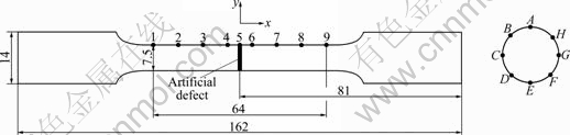
Fig. 3 Sketch map of specimen (Unit: mm)
3.2 Experimental results and analysis
3.2.1 Hp,y distribution surrounding specimen axis
As shown in Fig. 4, the Hp,y variation curve from Point A to Point H almost keeps steady at the process of fatigue. And the shape of curve is like what an inverse cosine function shows: Hp,y is the lowest at Point A, ascends from Point A to Point D, and descends from Point F to Point A. The values at Point C and Point G are almost equal, and the values at Point B and Point H are almost equal too.

Fig. 4 Hp,y distribution curve of eight points where N is cycle number: (a) Specimen a; (b) Specimen b; (c) Specimen c
When analyzing the stress distribution of the specimen in a cross section, it is found that the stress values of Points A-H are on an inverse cosine function curve, and the phase difference of two adjacent points is 0.25��. The stress distribution from Point A to Point H, and then to point A, is
![]() (8)
(8)
where ��0 is stress amplitude, and T is phase, T![]() [0, 2��].
[0, 2��].
Comparing the stress distribution with its Hp,y distribution, the conclusion is obtained. The Hp,y distribution is similar to the stress distribution, and it reflects the stress distribution.
3.2.2 MMM signals varied with cycle number at each point
As shown in Fig. 5, Hp,y at Points 1-9 gets steady after a few cycles, and the points at two sides of artificial defect have different variation laws. At early fatigue stage, Hp,y decreases to steady value at Points 1-4 and increases to steady value at Points 6-9. At late fatigue stage, Hp,y has a decreasing trend at Points 1-4 and has a increasing trend at Points 6-9, which obviously behaves in curves cross of Points 4, 5 and 6. In order to focus on the magnetic signal variation at Points 4-6, Hp,x at the three points is analyzed, as shown in Fig. 6. Hp,x at each point gets steady from disorder after a few cycles.
These phenomena have relationship with saturated stress variation in the process of fatigue. Since the stress of each point suffers changes according to cosine function, the stress-strain curve is a loop. For ductile solid, the variation of steady stress-strain hysteretic loop is shown in Fig. 7 [19]. There are three stages about the saturated stress variation: gradually increasing in a steady value at early fatigue stage, keeping steady, and continuing to increase at late fatigue stage. This variation law is similar to the variation law of the MMM signals.
3.2.3 Hp, y distribution along specimen axis
As shown in Fig. 8, the Hp,y distribution curve along the specimen axis almost keeps steady after about 100 cycles, and fluctuates at the middle position just before the specimen is broken. The set of steady curves are approximately central symmetry around the center points.
There is stress concentration around the artificial defect according to stress analysis. The center symmetric points of steady curves are all at the artificial defect, and the curve fluctuation before the specimen is broken happens around the artificial defect. So, the conclusion is obtained: the Hp,y-L curve can reflect the area of stress concentration, and display characteristic signal (the curve fluctuates at the area of stress concentration) before the specimen is broken.
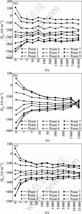
Fig. 5 Hp,y variation with N at Points 1-9: (a) Specimen a; (b) Specimen b; (c) Specimen c
4 Analysis and discussion using modified J-A model
Since the modified J-A model can describe the magnetomechanical effect well theoretically, it is used to analyze the experiment results above. Because the model parameters of this experimental material are unknown and need lots of work to be figured out, the parameters of Fig. 9 in Ref. [8] are taken for rough analysis in this work, and the stress range takes -100-100 MPa [8].

Fig. 6 Hp,x variation with N at Points 4-6: (a) Specimen a; (b) Specimen b; (c) Specimen c

Fig. 7 Stable stress-strain hysteresis loops
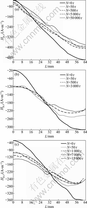
Fig. 8 Hp,y distribution along the specimen axis: (a) Specimen a; (b) Specimen b; (c) Specimen c
In addition, M in model is the magnetization intensity of the material. But the MMM field is the magnetic flux density on the surface of specimen, and there is a lift-off value between the surface of specimen and magnetic sensor usually. So, in order to character the MMM field more accurately, the calculation values of model should be multiplied by a coefficient f theoretically. And it should be 0.001-0.1 according to experience. However, the calculation values of model do not need to be multiplied by f for rough analysis in this work.

Fig. 9 M varying from Point A to Point H
4.1 Analysis of Hp,y distribution surrounding specimen axis
M changes with H0, �� and material parameters according to Eqs. (5) and (7). For a certain material that suffers elastic stress, only two factors (H0 and ��) are taken into account. And the values of H0 at Points A-H are the same, because these points are at the same cross section. So, the magnetic field variation is analyzed considering �� only.
It is known that the stress values of Points A-H are on an inverse cosine function curve, with phase difference of 0.25�� between two adjacent points. Consider the stress variation ��=-100cos(T) where T![]() [0, 2��], substitute it into Eqs. (5) and (7), let �š�=107, c��=0.08, and take the parameters of Fig. 9 in Ref. [8]. The M-T curve after the magnetizing field is steady and can be drawn up in Fig. 9 by Matlab software.
[0, 2��], substitute it into Eqs. (5) and (7), let �š�=107, c��=0.08, and take the parameters of Fig. 9 in Ref. [8]. The M-T curve after the magnetizing field is steady and can be drawn up in Fig. 9 by Matlab software.
Figure 9 shows that calculated M varying from Point A to Point H and then returning to Point A is not inverse cosine function shape as what the stress is. M ascends when 0��T��0.75��, descends when 1.25��T��2��, and has fall-and-rise phenomenon when 0.75��T��1.25��. However, the calculation result is similar to experiment result in curve shape except for some differences. The mainly differences are: The values of M at Point C and Point G are not equal according to calculation result, but the values of Hp,y at two points are almost the same according to experiment results; The calculated M at Point E is obvious lower than that at Point E and Point F, which is also different from experiment results.
These differences can be explained clearly. The magnetic signal collected by the sensor at a point is not only the signal produced by this point, but the part that lots of adjacent points produce and manifest at this point. According to the calculation result, the value of M at points around Point C is similar to that at Point G. So, the magnetic signals collected at two points are the same. The value of M at points around Point E is all higher than that at Point E, so the magnetic signal collected at point E is higher than calculated result of model. According to this idea, the collected M values at eight points are figured out roughly in Fig. 9. And it is more similar to experiment results compared with the M-T curve calculated from the model.
4.2 Analysis of MMM signal varying with time at process of fatigue
The change of maximum stress amplitude at the process of fatigue is shown in Fig. 7 for ductile solid (including metal material), but the expression of change law is unknown. In order to research the MMM signal changes at the process of fatigue using modified J-A model, the expression of maximum stress amplitude changes at three fatigue stages are supposed to be
 (9)
(9)
where ��0 is the original maximum stress amplitude, n![]() [0,11] stands for the whole life of material, n
[0,11] stands for the whole life of material, n![]() [0,1] means the early fatigue stage, n
[0,1] means the early fatigue stage, n![]() [1,10] means the middle stage of fatigue, and n
[1,10] means the middle stage of fatigue, and n![]() [10,11] means the late fatigue stage.
[10,11] means the late fatigue stage.
Substitute Eq. (9) into Eqs. (5) and (7), let �š�=107, c��=0.08, ��0=-1��108 Pa, and take the parameters of Fig. 9 in Ref. [8]. A series of M-n curves are obtained, as shown in Fig. 10. Under the condition of positive external magnetic field, M changes greatly as the stress changes at the first stage of fatigue, keeps steady at the second stage, and decreases greatly at the third stage of fatigue. M changes inversely when the external magnetic field is negative.
The simulation results can explain the experiment results well. For the PQ1-6 pure bend fatigue experiment machine used in this experiment, the chucks rotate with specimen and are magnetized by the geomagnetic field. So, in this experiment, H0 is not the geomagnetic field only, but is mainly the field caused by two chucks. As shown in Fig. 11, (H0)y distribution along the specimen is an oblique line with negative slope. (H0)y is positive at Points 1-4, and is negative at Points 6-9. And (H0)x is positive at Points 4-6. So, Hp,y variation with N coincides with experiment results in Fig. 6. The Hp,y values of Points 1-9 ranking from large to small is because the (H0)y values of these points rank from large to small. The Hp,x variation law of Points 4, 5 and 6 can be explained in the same way. The drastic change at the first few cycles is because the initial Hp,x value is higher or lower than the steady value, as shown in Fig. 11.

Fig. 10 M-n curves

Fig. 11 Magnetizing field of chucks
4.3 Analysis of Hp,y distribution along specimen axis
Stress concentration exists around the artificial defect under applied load. And according to the Saint Venant��s principle, the stress distribution will not be influenced by artificial defect where the distance from artificial defect is larger than specimen diameter. The normal distribution function f(x)=1/[�ġ�(2��)1/2]�� exp[-(x-��)2/(2��2)] is chosen to describe the stress concentration effect. Take ��=32 and ��=7.5/3=2.5 to insure the stress distribution 7.5 mm away from the defect center not effected by artificial defect. And the stress distribution from Point 1 to Point 9 is given by Eq. (10), where 0��l��64, ��0 is the stress without stress concentration influence, 1+0.16k=K, and K is stress concentration factor of artificial defect.
![]() (10)
(10)
Substitute Eq. (10) into Eqs. (5) and (7), let �š�=107, c��=0.08, K=2.75, ��0=-1��108 Pa, take (H0)y=-5(l-32) into Man, and take the parameters of Fig. 9 in Ref. [8]. A series of My-L curves are obtained in Fig. 12. My keeps steady when its position is far away from artificial defect, and changes drastically in the region with stress concentration. And My-L curve passes through zero at the point with maximum stress, which coincides with initial MMM principle put forward by DUBOV [1] that the MMM signal in normal direction passes through zero at the region of stress concentration.
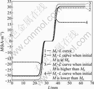
Fig. 12 My-L curves
The simulation results can explain the experiment results well. The signal collected by sensor includes By caused by stress (By=f��My), and Be,y caused by chucks, geomagnetic field and other environmental magnetic field, as shown in Fig. 13. Theoretically speaking, the Hp,y-L curve should fluctuate at the region of stress concentration. However, because of the lift-off effect, By collected by the sensor is weak, the Hp,y-L curve fluctuation is difficult to see except that the crack is obvious and the stress concentration is serious. So, in this experiment, the Hp,y-L curve fluctuation can be seen only before the specimen is going to be broken.

Fig. 13 Theoretical Hp,y-L curve
5 Conclusions
1) In MMM detection, the magnetization of material would irreversibly approach to the local equilibrium state M0 instead of the global equilibrium state Man. The M0-�� curve is a loop around the Man-�� curve, and it changes with cycle load type.
2) The modified J-A model is constructed by replacing Man in J-A model with M0 and changing some parameters, and it can describe the magnetomechanical effect at low external magnetic field better than the J-A model.
3) In the rotating bending fatigue experiments, the MMM field in normal direction around cylinder specimen is in inverse cosine function shape, which coincides with the calculation result of modified J-A model after some necessary modifications.
4) The MMM field variation at a certain point is divided into three stages with the variation of stable stress-strain hysteresis loop in fatigue process. The calculation result of modified J-A model can not only explain the three stages of MMM field changes, but also explain the different change laws when the applied magnetic field and initial magnetic field are different.
5) The MMM field distribution in normal direction along specimen axis reflects stress concentration effect at artificial defect, and the magnetic signal fluctuates around the defect at late fatigue stage. Taking stress distribution function nearby the artificial defect into modified J-A model, the calculation results coincide with the initial MMM principle, and can explain the signal fluctuates around the defect.
6) Mechanism research, experiment results and model calculation results all show that the MMM field is sensitive to the variation of stress. The modified J-A model can explain experiment results well, and it is fit for MMM detection. However, the M value in model is the magnetization intensity inside the material, the MMM field is the magnetic flux density on the surface of specimen, and there is a lift-off value between the surface of specimen and magnetic sensor usually. So, in order to character the MMM field more accurately, the calculated value of model should be multiplied by a coefficient f which needs to be figured out.
References
[1] DUBOV A A. A study of metal properties using the method of magnetic memory [J]. Metal Science and Heat Treatment, 1997, 39(9/10): 401-405.
[2] DUBOV A A, KOLOKOLNIKOV S. Comprehensive diagnostics of parent metal and welded joints of steam pipeline bends [J]. Welding in the World, 2010, 54(9/10): R241-R248
[3] ROSKOSZ M, GAWRILENKO P. Analysis of changes in residual magnetic field in loaded notched samples [J]. NDT&E International, 2008, 41(7): 570-576.
[4] YAN Chun-yan, LI Wu-shen, DI Xin-jie, XUE Zhen-kui, BAI Shi-wu, LIU Fang-ming. Variation regularity of metal magnetic memory signals with inspecting time-interval and location [J]. J Cent South Univ Technol, 2007, 14(3): 319-323.
[5] JIAN Xing-liang, JIAN Xing-chao, DENG Guo-yong. Experiment on relationship between the magnetic gradient of low-carbon steel and its stress [J]. Journal of Magnetism and Magnetic Materials 2009, 321(21): 3600-3606.
[6] XU Ming-xiu, WU Da-bo, XU Min-qiang, LENG Jian-cheng, LI Jian-wei. The MMM detection of rotating bending fatigue damage for 45QT steel [J]. Advanced Science Letters, 2011, 4(1-6): 1-6.
[7] JILES D C, ATHERTON D L. Theory of ferromagnetic hysteresis [J]. Journal of Magnetism and Magnetic Materials, 1986, 61: 48-60.
[8] JILES D C. Theory of the magnetomechanical effect [J]. Journal of Physics D: Applied Physics, 1995, 28(8): 1537-1546.
[9] RAGHUNATHAN A, MELIKHOV Y, SNYDER J E, JILES D C. Generalized form of anhysteretic magnetization function for Jiles-Atherton theory of hysteresis [J]. Applied Physics Letters, 2009, 95(17): 172510.
[10] SQUIRE P T. Magnetomechanical measurements and their application to soft magnetic materials [J]. Journal of Magnetism and Magnetic Materials, 1996, 160(1): 11-16.
[11] LENG Jian-cheng, XU Min-qiang, XU Ming-xiu, ZHANG Jia-zhong. Magnetic field variation induced by cyclic bending stress [J]. NDT&E International, 2009, 42(5): 410-414.
[12] SABLIK M J, WILHELMUS J G, SMITH K, GREGORY A, CLAYTON M, PALMER D, BANDYOPADHYAY A, FERNANDO J G, MARCOS F C. Modeling of plastic deformation effects in ferromagnetic thin films [J]. IEEE Transactions on Magnetics, 2010, 46(2): 491-494.
[13] LI Hui-qi, LI Qing-feng, XU Xiao-bang, LU Tie-bing, ZHANG Jun-jie, LI Lin. A modified method for Jiles-Atherton hysteresis model and its application in numerical simulation of devices involving magnetic materials [J]. IEEE Transactions on Magnetics, 2011, 47(5): 1094-1097.
[14] MAKAR J M, ATHERTON D L. Effects of isofield uniaxial cyclic stress on the magnetization of 2% Mn pipeline steel-behavior on minor hysteresis loops and small major hysteresis loops [J]. IEEE Transactions on Magnetics, 1995, 31(3): 2220-2227.
[15] XU Ming-xiu, XU Min-qiang, LI Jian-wei, LENG Jian-cheng, ZHAO Shuai. In service detection of 45 steel��s rotary bending fatigue damage based on metal magnetic memory technique [J]. Advanced Materials Research, 2010, 97-101: 4301-4304.
[16] DONG Li-hong, XU Bin-shi, DONG Shi-yun, CHEN Qun-zhi, WANG Dan. Monitoring fatigue crack propagation of ferromagnetic materials with spontaneous abnormal magnetic signals [J]. International Journal of Fatigue, 2008, 30(9): 1599-1605.
[17] YANG En, LI Lu-ming, CHEN Xing. Magnetic field aberration induced by cycle stress [J]. Journal of Magnetism and Magnetic Materials, 2007, 312(1): 72-77.
[18] CRAIK D J, WOOD M J. Magnetization changes induced by stress in constant applied field [J]. J Phys D: Appl Phys, 1970, 3(7): 1009- 1016.
[19] SUBRA S. Fatigue of materials [M]. Cambridge: Cambridge University Press, 2003: 27-29.
(Edited by DENG L��-xiang)
Foundation item: Projects(11072056, 10772061) supported by the National Natural Science Foundation of China; Project(A200907) supported by the Natural Science Foundation of Heilongjiang Province, China; Project(20092322120001) supported by the PhD Programs Foundations of Ministry of Education of China
Received date: 2011-04-06; Accepted date: 2011-07-22
Corresponding author: XU Ming-xiu, PhD candidate; Tel: +86-451-86414479; E-mail: xmxyippee@gmail.com
Abstract: In order to propel the development of metal magnetic memory (MMM) technique in fatigue damage detection, the Jiles-Atherton model (J-A model) was modified to describe MMM mechanism in elastic stress stage. A series of rotating bending fatigue experiments were conducted to study the stress-magnetization relationship and verify the correctness of modified J-A model. In MMM detection, the magnetization of material irreversibly approaches to the local equilibrium state M0 instead of global equilibrium state Man under cyclic stress, and the M0-�� curves are loops around the Man-�� curve. The modified J-A model is constructed by replacing Man in J-A model with M0, and it can describe the magnetomechanical effect well at low external magnetic field. In the rotating bending fatigue experiments, the MMM field distribution in normal direction around cylinder specimen is similar to the stress distribution, and the calculation result of model coincides with experiment result after some necessary modifications. The MMM field variation with time at a certain point in fatigue process is divided into three stages with the variation of stable stress-stain hysteresis loop, and the calculation results of model can explain not only the three stages of MMM field changes, but also the different change laws when the applied magnetic field and initial magnetic field are different. The MMM field distribution in normal direction along specimen axis reflects stress concentration effect at artificial defect, and the magnetic signal fluctuates around the defect at late fatigue stage. The calculation results coincide with the initial MMM principle and can explain signal fluctuates around the defect. The modified J-A model can explain experiment results well, and it is fit for MMM field characterization.
