

J. Cent. South Univ. (2020) 27: 2291-2310
DOI: https://doi.org/10.1007/s11771-020-4450-7

A model to determining the remaining useful life of rotating equipment, based on a new approach to determining state of degradation
Saeed RAMEZANI1, Alireza MOINI1, Mohamad RIAHI2, Adolfo Crespo MARQUEZ3
1. Department of Industrial Engineering, Iran University of Science and Technology, Tehran, Iran;
2. Department of Mechanical Engineering, Iran University of Science and Technology, Tehran, Iran;
3. Department of Industrial Management, University of Seville, Spain
 Central South University Press and Springer-Verlag GmbH Germany, part of Springer Nature 2020
Abstract:
Condition assessment is one of the most significant techniques of the equipment��s health management. Also, in PHM methodology cycle, which is a developed form of CBM, condition assessment is the most important step of this cycle. In this paper, the remaining useful life of the equipment is calculated using the combination of sensor information, determination of degradation state and forecasting the proposed health index. The combination of sensor information has been carried out using a new approach to determining the probabilities in the Dempster-Shafer combination rules and fuzzy c-means clustering method. Using the simulation and forecasting of extracted vibration-based health index by autoregressive Markov regime switching (ARMRS) method, final health state is determined and the remaining useful life (RUL) is estimated. In order to evaluate the model, sensor data provided by FEMTO-ST Institute have been used.
Key words:
Cite this article as:
Saeed RAMEZANI, Alireza MOINI, Mohamad RIAHI, Adolfo Crespo MARQUEZ. A model to determining the remaining useful life of rotating equipment, based on a new approach to determining state of degradation [J]. Journal of Central South University, 2020, 27(8): 2291-2310.
DOI:https://dx.doi.org/https://doi.org/10.1007/s11771-020-4450-71 Introduction
Prognostics and health management (PHM) concept are retrieved from the well-known maintenance and diagnosis techniques such as preventive maintenance (PM), reliability centered maintenance (RCM) and especially condition-based maintenance (CBM) [1]. CBM consists of data gathering and processing (condition monitoring), so that, based on the analyzed information, maintenance decisions are taken and as a result the unnecessary maintenance measures are prevented. PHM could be considered as a developed form of CBM. CBM techniques can provide the input of prognostic model in PHM. Failure mechanism analysis in PHM (corrosion, fatigue, overload, etc.) is related to the product life cycle management. Because of the ability to assess health states and forecasting failures, PHM can even be considered the foundation of modern techniques in the field of maintenance [2]. In general, three different approaches to determining the state of equipment degradation are presented by the researchers: data-driven, physics of failure and hybrid method [3]. Data-driven approach can be interpreted as black box that studies the behavior of the system directly from the collected data (such as a vibration, noise, emission, force, pressure, etc.). The approach is based on this idea as long as the system does not fail, the extracted features of the sensor data will not be changed. In this approach, the unprocessed data of system monitoring is converted to appropriate information and behavioral models. Since these methods are based on data trajectory, they are strong in forecasting the future behavior of equipment, especially the end of life phase [4]. Many researches have been conducted on data-driven approaches to estimate the remaining useful life (RUL). Diversity in artificial intelligence, machine learning, and statistical methods to determine degradation and forecaste how long failure would take, has developed different processes to calculate the RUL. For example RAI et al [5] have investigated a variety of methods according to the type of equipment (bearing, shafts, gears, pumps and alternators). The most critical part in rotary machinery is rolling element bearing and comprises 45%-55% of these equipment failures [5]. We focus on forecasting bearing remaining useful life based on a data-driven approach in this paper.
Despite the advantages of a data-driven approach, sometime extracted information can be misleading and make decision-making difficult. Especially when there are several sources of information (sensors), how to use information individually and in combination is challenging [6]. On the other hand, the presence of non-linear and non-smooth trajectories with shock is usually one of the characteristics of the information obtained from sensors in mechanical equipment [7]. In this paper, we focus on these two issues. To do this, we present a data-driven method to determine the degradation state of rolling element bearings, by combinating the sensor information. The proposed method is based on the combination rules of Dempster-Shafer theory and clustering. We also use the autoregressive Markov regime switching method to model nonlinearity along with regime change in extracted data.
The rest of paper is organized as follows. In Section 2, the works related to determining the RUL of rolling element bearings are presented. In Section 3, the proposed method is described. In Section 4, the results of model implementation for experimental data are presented and Section 5 concludes the paper.
2 Related works
In recent years, many studies have been conducted on the diagnosis of degradation state and the determination of the RUL using a data-driven approach for rotating equipment, especially rolling element bearings. Meanwhile, vibration data has the largest share in the analysis of this equipment. This study also focuses on sensor vibration data, and related studies on the failure analysis and the RUL estimation using vibration data have been investigated. In general, in the data-driven approach, the process of determining the RUL is performed in three steps: selecting a health index (HI) to track the health/degradation state; determining the state of health/degradation state; estimating the RUL using forecasting methods, HI and time-to-failure.
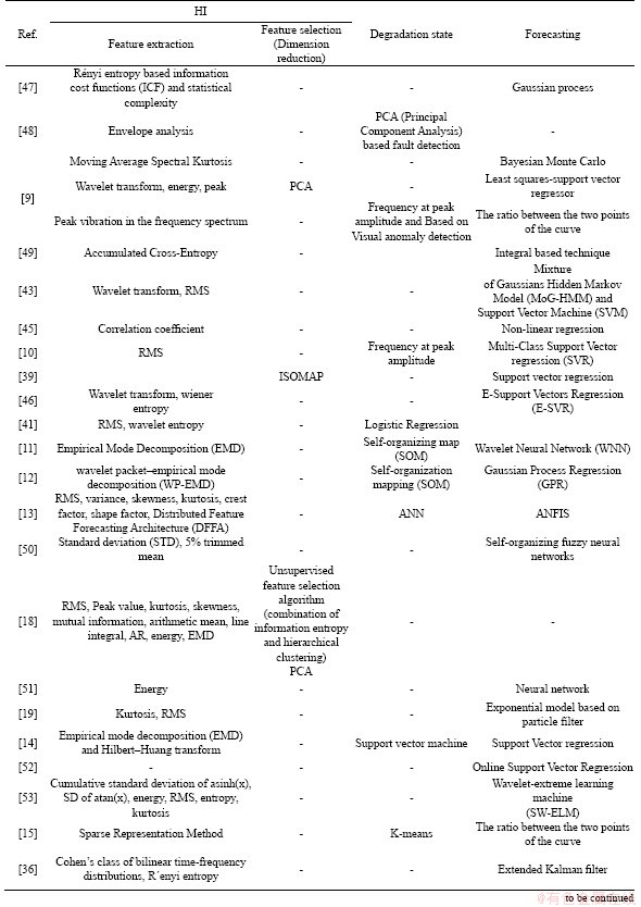
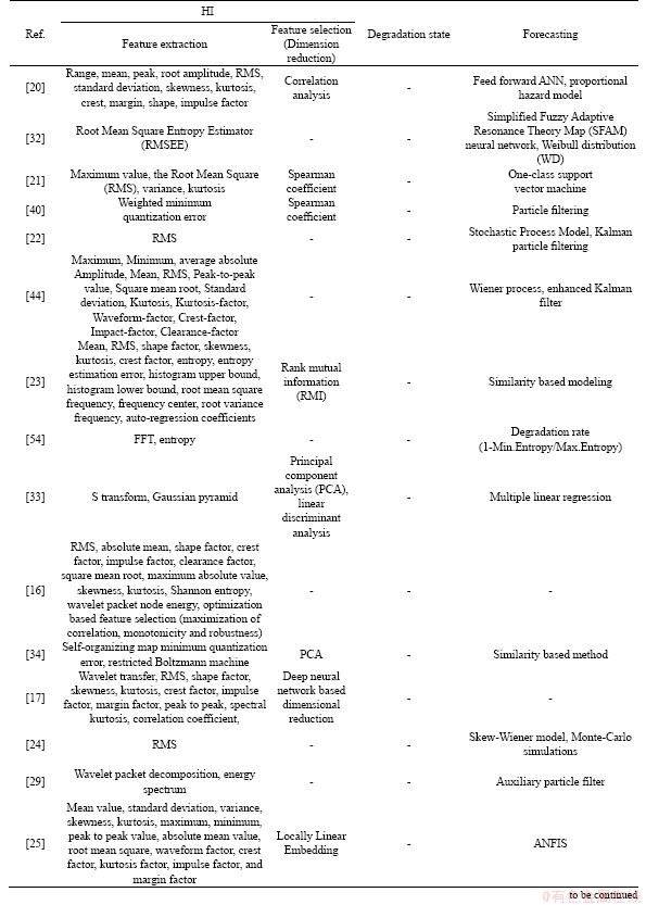
Researchers often formulate their own research according to these three steps. In Table 1, the methods used by the researchers, are presented according to each of the above steps. Some researches, such as [8-15], provided the framework in which the three-step analysis to determine the RUL are examined, while in some, only one of the steps is considered. For example, in Refs. [16, 17] only methods for determining an appropriate HI are presented.
In the first step of the data-driven approach, researchers are looking for an index that represents the health state of the equipment, so that it can detect the degradation by tracking it and estimating the RUL of the equipment with its forecasting. Generally, this step involves two stages: feature extraction and feature selection. In some researches, the classical time domain features such as mean, standard deviation, kurtosis, RMS [9, 10, 13, 16, 18-27], the frequency domain such as the maximum amplitude in the frequency band [28] or the frequency-time domain like the wavelet transform features has been used [29], while some other studies suggest to use new features [30-36]. Also, in some studies, feature selection and dimension reduction methods, such as PCA, ISOMAP, and other more advanced methods have been used to enhance the data clustering, increasing explanatory power of independent variables and reducing the complexity of the data, such as [9, 17, 18, 20, 21, 26, 27, 34, 37-39].
In the second step, the equipment degradation state is determined using the current state of the HI and the information obtained from the recorded historical data set (learning set). Since there is no prior information about the exact boundary of degradation states, unsupervised learning methods, such as clustering with the arbitrary number of clusters are used to determine the degradation state [11-15]. Peak frequency variations and its visualization [9, 10] and the occurrence of anomaly in the HI [40] are considered as signs to change the state of degradation. In Ref. [38], a matter-element model based on the correlation coefficient between the current state and the healthy state is presented to determine the degradation state of equipment.
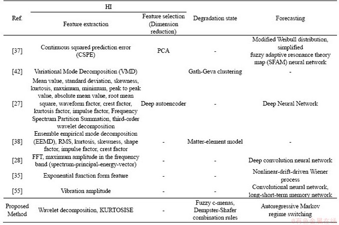
Table 1 Research related to determining RUL of rolling element bearings
Continued
Continued
In the third step, the RUL is estimated by using three different approaches: 1) fitting a statistical model; 2) training an intelligent forecaster based on the existing historical data set for model fitting; 3) training. In the first approach, the forecasted variable is the HI. In this case, the forecasting horizon is considered equivalent to a predetermined threshold, and the time until the index reaches this threshold is determined as the RUL [12, 22, 24, 36, 40, 41]. In the second approach, the time-to-failure variable is considered as a dependent variable or target, and on this basis, the forecasting model is fitted or trained. In this case, the result of forecasting is an estimate of RUL [9-11, 13, 14, 21, 33, 37, 39, 42-45]. In the third approach, RUL is estimated by identifying the learning dataset which is most similar to the sample being tested and creating a fit between the HI in different degradation states [9, 15, 23, 34, 46].
In this paper, all the three steps mentioned above are used to determine the remaining useful life. In the first step, a new feature called Kurtosis-Entropy (KURTOSISE) is introduced and its predictability is evaluated. In order to determine the degradation state, a new method which combines the fuzzy c-means clustering and Dempster-Shafer theory is used. In the proposed method, the degradation states are determined based on each of the sensors and using fuzzy c-means clustering. The obtained degradation states are combined by using the combination rules of the Dempster-Shafar theory and the degradation state of the equipment is determined. Finally, the remaining useful life is estimated by predicting the HI using the autoregressive Markov regime-switching model which has never been employed for this purpose before. In the next section, the proposed method is explained in detail.
3 Proposed method
The framework of proposed method in this paper is similar to the researches mentioned in the previous section, consisting of three steps: determining the HI, determining the degradation state and finally, forecasting the RUL of the equipment. In this method, the run-to-failure data set is needed to calculate the RUL of the new bearing based on the characteristics of these data (ball bearing vibration data sets). Figure 1 illustrates the procedure of the proposed method to determine the RUL of the equipment.
As seen in Figure 1, the process of estimating the RUL is accomplished in two general phases: learning phase and testing phase. In the following, the methods and how they are used in each of these two phases are described separately.
3.1 Learning phase
3.1.1 Signal decomposition
In the first step of HI determination, vibration signals are transformed and de-noised by wavelet decomposition. In Ref. [56], for vibration signal decomposition by wavelet, it is recommended to use the third to fifth levels of Daubechies wavelets, and in this paper, the fourth level of Daubechies wavelet (D4) for vibration signal decomposition is used.
3.1.2 Feature extraction
In the second step of HI determination, a new feature is extracted from decomposed signals. RMS and kurtosis are the most useful feature for vibration signal analysis [57]. One of the limitations of these two, in particular for approximation of the RUL, is their sharp fluctuations before complete failure. Heavy noises are rampant in the fault information at the initial stages of bearing failures [58]. To deal with this problem, we suggested Kurtosis-Entropy method:
 (1)
(1)
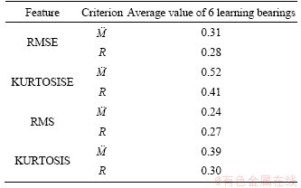
where n is the length of sliding window. This feature, in the final state of failure, which is associated with severe fluctuations, shows a more smooth behavior. Additionally, eliminates the sudden raises in kurtosis features when it eventually reaches its failure. The proposed feature is similar to the feature presented in Ref. [32] with the difference that instead of RMS, Kurtosis is used. For a successful HI forecasting, trendability and monotonicity of HI are two main criteria [59]. Using experimental data, details of which are described in Section 4.1, four features (kurtosis, RMS, RMSE and KURTOSISE) based on two mentioned criteria are compared and KURTOSISE showed a better performance. The details of this analysis are presented in Table 2.
3.1.3 Removing outliers and smoothing
In the final step of determining the HI, Hample filter and a moving average filter is used respectively to remove outliers and smooth the path of features, respectively.
In Hample filter, for each sample of x, the median of a window comprising the sample and its six adjacent samples (three per side) is calculated. Also the standard deviation of each sample about its window median is approximated using the median absolute deviation. A sample is replaced with the median, if it has three standard deviations or more difference with median [60].
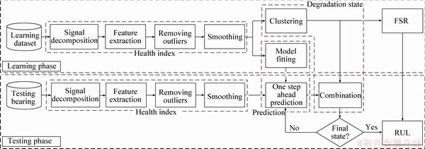
Figure 1 Proposed method procedure
Table 2 Trendability and monotonicity of RMSE and KURTOSISE features
Also, the moving average filter for a series of data is calculated as follows:
 y(i+N-1)+��+y(i-N)) (2)
where y(i) is the smoothed i-th data; N is the number of adjacent data in each side of y(i) and 2N+1 is the size of time window [61].
3.1.4 Clustering
To determine the degradation states, the HI is clustered. Each cluster represents each of the degradation states. Lower boundary of final cluster with the highest HI value indicates complete failure and is defined as the threshold of forecasting. In the proposed method, the combination of data to determine the state (cluster) of degradation is determined by the probability of belonging to these clusters. This probability is obtained by proximity to cluster centers. For this reason, fuzzy c-means (FCM) algorithm, which is a centroid based algorithm, has been used, and the details of the combination method are explained in Section 3.2.2. FCM is one of the clustering methods that allows each data set to belong to several clusters with different membership degree [62]. In this method, clustering is done by minimizing Jm:
 (3)
(3)
where D is the number of data; N is the number of clusters; m is any real number greater than 1 (m>1); xi is the i-th data; cj is the center of cluster j and ��ij is the degree of membership of xi in cluster j. For a certain data xi, the total value of membership for all clusters is one. FCM clustering is done by taking the following steps:
1) Initial ��ij are randomly assigned. By using Eq. (4), the centers of the clusters are calculated:
 (4)
(4)
2) ��ij is updated according to Eq. (5).
 (5)
(5)
3) Objective function Jm is calculated. This process is repeated until Jm becomes smaller than a predetermined threshold or reaches a specified iteration number.
3.1.5 Fitting forecasting model
As outlined in Section 2, there are generally two approaches to forecaste. Here we use the first approach and fit a autoregression model for the HI.
Recently, significant improvements have been achieved in order to capturing the non-linear structure and transient behavior of time series data. Examples of such non-linear and non-stationary time series are consisted of acoustic emission from manufacturing machinery and structural systems, customer demand, production rates in a manufacturing company, electricity load in a smart grid, traffic at a node (intersection) across transportation and telecommunication networks, stock prices and other market indices, electroencephalogram (EEG) and electrocardiogram (ECG) signals, and temperature and other weather signals [63]. Examples of using classic models in prognostics included exponential smoothing [64], autoregressive models [65-69]. Also, non-linear models have been used in this field, for example neural network and deep neural network models [55, 63, 70-72], extended Kalman filter [36, 73, 74] and regime-switching models [75, 76][16].
In the proposed method of this study, autoregressive Markov regime switching model (ARMRS) has been used to forecast the HI. This model was first introduced by HAMILTON [77] and is one of the most famous non-linear time series models. The major application of this method is in search of economic volatility and regime change as a result of changes in monetary policy, domestic and international finance in countries or shocks such as natural disasters, war and etc. The reason for using this approach is its ability to model changes of mean and volatility of HI. Generally, regime change in the HI time series is caused by the equipment��s degradation process which occurs because of such damages as fatigue, cracks, spall, etc.
In Markov regime switching, the states is divided into k states which St is t-th state (t=1, 2, ��, k), and any state may express a regime change. As St could be a state that has occurred at time t, resulting in the intended change of variables (for example Yt). So based on Markov property it could be written (P is probability):
 (6)
(6)
Now consider the following process:
 (7)
(7)
where St=1, ��, k and ��t follows a normal distribution with zero mean and variance  This is the simplest case of a model with a dynamic change. In this process, there is regime change ability to intercept �� and variance ��2 according to variable St. Now assume that process in Eq. (7) has two regimes (k=2). One way to illustrate this state is as follows:
 (8)
(8)
where 
This style of writing, easily depicts the two processes for dependent variable yt. Different volatility  and
and  in every regime, shows an uncertainty in every regime. In Markov regime switching, the change of regime is random. However, the available dynamic in a switching process is determined by a transfer matrix. This matrix controls the probability of a change from one regime to another and is illustrated as follows:
 (9)
(9)
where pij is the probability of switching from regime i to regime j. In this study, we used the maximum likelihood method to estimate the model parameters [77]. Assume the below regime change:
 (10)
(10)
The log-likelihood of the model is determined as follows:
 (11)
(11)
If all of the world regimes are known then St will be available and estimating the model by maximum likelihood will also be easy. but we know that these regimes are unknown for us. Assuming that f(yt|St=j, ��) is likelihood function for regime j for a set of �� parameters, then the full log-likelihood function for the model is determined as follows:
 (12)
(12)
Equation (12) is actually weighted likelihood function, where weights determined by regimes probabilities. Since these probabilities are not observable, we cannot directly use Eq. (12). However, based on available information, we could have a deduction from it. This is Hamilton��s filter main idea to calculate filtered probabilities based on the new information for any regime. Supposing that ��t-1 is the available information matrix at t-1, then using Hamilton��s filter, P(St=j) will be calculated by below iterative algorithm (for two regimes):
Step 1: Make a guess for initial probabilities (t=0) of every regime P(S0=j) for j=1, 2. Then we have:
 (13)
(13)
 (14)
(14)
Step 2: Put t=1 and calculate the probabilities for every regime based on information until t-1:
 (15)
(15)
Step 3: Update the parameters and transition probability  of each regime with new information from time t. Use the below formula according to the new information to update the probability of each regime.
 (16)
(16)
Put t=t+1 and repeat steps 2 to 3 until t=T. In this case, a set of filtered probabilities is obtained for each regime with t from 1 to T. The outlined steps provide the possibility to maximizing the log-likelihood Eq. (12) and estimating the parameters.
A Markov regime switching model can be generally regressive with exogenous and autoregressive variables as follows:


 (17)
(17)
This Markov regime change model offers a wide variety of different modes. NnSe and NnSa illustrate the number of coefficients without regime change for exogenous and autoregressive variables, respectively. Also, NSe and NSa show the number of coefficients with capability for regime change. Additionally, includes all exogenous variables without the regime change effect and
  includes all autoregressive variables without regime change;
 is the term given error probability density function with parameters (
 ) that have the capability of regime change and ��i, ��j, ��k and ��z are the coefficients. In this study, we used ARMRS model with no exogenous variable. Ability to regime change for autoregressive variables (AR) and volatility has also been considered. We used Bayesian information criterion (BIC) [78] to determine AR lags and Perlin��s MATLAB package [79] for estimating the parameters of ARMRS model.
3.1.6 FSR determination
Often, the HI behaves with severe fluctuations near complete failure which indicates the final state (cluster) of equipment degradation. For this reason, forecasting based on autoregression models may not be accurate in the final state. To solve this problem, we use the ratio between final cluster and run-to-failure time that we call it final state ratio (FSR, rF). The idea of using state ratios to forecast was used earlier in Ref. [9].
Assuming that the repetition of the degradation state pattern of historical data (bearing learning data) at future, the final state ratio defined as follows:
 (18)
(18)
where tEnd is run-to-failure time and tFS is the entrance time to the final cluster Figure 2. In the learning phase, rF is calculated for each bearing and is used to predict the duration of the final cluster in the testing phase, and this process is described in Section 3.2.3.
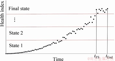
Figure 2 Run-to-failure time and time to entrance final cluster
3.2 Testing phase
In the testing phase, the RUL for each of the bearings is calculated. To this end, the HI, similar to the learning phase, is calculated for the bearings, and then the degradation state is determined by forecasting the HI obtained from the horizontal and vertical sensor vibration and their combination. This process will continue to reach the final cluster. The process of forecasting and combination is described below.
3.2.1 One step ahead forecasting
In this phase, considering t as the current time, HI is simulated by Markov regime switching for t+1. The forecasting process is performed using models that fit into learning data in the learning phase. Therefore, if there are N learning samples, the forecasting process is performed taking into account the models fitted to these N samples.
3.2.2 Combination
In this section, first, a preliminary is presented about the theory of evidence, and then the method for using it to combine the features of the problem is described. Dempster presents the mathematical theory of evidence, and SHAFER developed it [80]. This theory is important in discussing existing beliefs about a state or system of states. Beliefs about states are not the same, but, with the help of this theory, the available evidence from this state could be combined. Further, the rules of combination are presented in Ref. [81].
Principal function in Dempster-Shafer theory is bpa, which is represented by m and indicates the power set in a (0,1). The bpa for the subsets of the power set is 1 and for the null set is 0. bpa for a specific set A (represented by m(A)), expresses the proportion of all relevant and available evidence that supports the claim that a particular element of X (the universal set) belongs to the set A but is not a particular subset of A [82]. m(A) does not have any claims about any other subset of A and is related only to the set A. Any further evidence on the subsets of A shall be represented by another bpa, i.e. B A. The bpa for the subset B is m(B). Formally, this description of m can be represented with the following three equations:
m:P(X)��[0, 1] (19)
m(f)=0 (20)
 (21)
(21)
where P(X) indicates the power set of X; f is the null set and A belongs to power set (A��P(X)).
The Dempster rule of combination is purely a conjunctive operation (AND). The combination rule results in a belief function based on conjunctive pooled evidence. Particularly, in this matter the combination of two bpas m1 and m2 (called the joint m12) is computed in the following manner:
 (22)
(22)
 (23)
(23)
 (24)
(24)
where k indicates the basic probability mass related to conflict. When the intersection is null, k is calculated by sum of the products of the bpas of all sets. The denominator in Dempster��s rule, 1-k, is a normalization factor. It leads to the complete negligence of conflict and attributes any probability mass related to the conflict to the null set.
Here, in order to fusing the degradation states, each sensor is considered as a source of information. The probability that the system will be assigned to each fault state is calculated based on the equipment feature distance from the predetermined cluster center for failures. According to presented descriptions about Dempster-Shafer theory, suppose that n sensors are connected to the machine which reports the degradation information plays the role of observer (E1, ��, En) (for example for the horizontal and vertical sensor). Also suppose that C={c(1), c(2), ��, c(k)} is the cluster centers (k clusters) that are obtained by the fuzzy c-means algorithm for all of the learning data sensors. In this case, the probability of belonging HI in time t (HIt of n-th sensor, to j-th cluster (the bpa for the subset c(k)) is considered as follows:
 (25)
(25)
where D(HIt, c(j))=|HIt-c(j)| is the distance of HIt from the center c(j) (Figure 3). Therefore, for each HIt of n-th sensor, the probability belonging to k-th cluster can be obtained using the Eq. (25). Finally, HIt belongs to the cluster that has the highest m1, ��, n(c(k)), where according to Eq. (22), m1, ��, n(c(k)) is joint bpa of all n sensors.
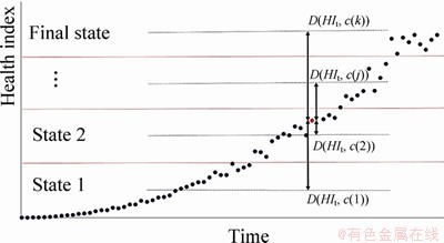
Figure 3 Data point distance from clusters
3.2.3 RUL estimation
After determining the state (cluster) of the forecasted HI using the presented combination method, if we reach the final cluster, then combined with Eq. (18), RUL can be calculated as follows:
 (26)
(26)
where tc is the current time (RUL calculation time) and Tt is the time to the final cluster (threshold) (Figure 4).
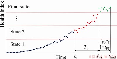
Figure 4 RUL estimation process
4 Experiment
4.1 Dataset
To evaluate the proposed procedure, the experimental bearing degradation dataset provided by FEMTO-ST Institute was used in Ref. [83]. According to this dataset, the data has been considered with three different loads:
1) First operating condition: 1800 r/min and 4000 N;
2) Second operating condition: 1650 r/min and 4200 N;
3) Third operating condition: 1500 r/min and 5000 N.
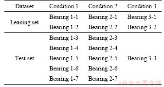
For this estimation, six run-to-failure datasets have been provided for forecasting models and RUL estimation for 11 other bearings have been run-to-failure data (Table 3). Vibration signals (horizontal and vertical) and temperatures have been collected for all testing steps. There is no information about the origins and roots of failure (the balls, the inner ring, the outer ring, the cage, etc.).
Table 3 FEMTO-ST institute dataset
4.2 Learning phase results
In the learning phase, the initial processing of data for all learning bearing vibrations (bearing 1-1, 1-2, 2-1, 2-2, 3-1, 3-2) has been performed. In Figure 5, the main signal (at the top of the figure), the decomposed signal by fourth level of D4 wavelet (in the middle of the figure) and the extracted feature smoothed by the moving average filter (at the bottom of the figure), are shown for bearing 1-1.
Using fuzzy c-means method and considering four clusters, as four stages of bearing degradation (health state to complete failure), cluster centers has been achieved in every condition for each learning (horizontal and vertical sensor) bearing. After getting cluster centers, the states obtained by horizontal and vertical HIs of each bearing could be combined. For this purpose, the combination rule of Dempster-Shafer theory has been used. For example, Figure 6 exhibits both horizontal and the combination of their states (cluster) for bearings 1-1 and 1-2.
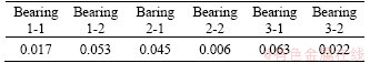
By clustering all the learning bearings in different conditions, FSR has been calculated for each one of the bearings by Eq. (19) (Table 4).
After determining FSR, the ARMRS model is fitted for all the learning bearings, considering 1 to 3 lags in the model. By using BIC, the best lag for each fitted model is selected (the results of lag selection are in Table 5).
4.3 Testing phase results
In the testing phase, the degradation states of the testing bearings are initially determined using the proposed clustering method. ARMRS simulation has been used to forecast the Tt and RUL according to Eq. (26). The Monte Carlo simulation has been done for 100 paths for each data point of paths, degradation state (cluster) and Tt were determined. Given the probability mass function obtained from the forecasted Tt, the final Tt is calculated based on three cut-off levels of 10%, 50% and 90%, respectively. Also for each testing bearing, two RULs were calculated considering the two learning bearing in each condition.
To evaluate the proposed combination method, the forecasted results are compared in the following three cases:
1) Horizontal sensor;
2) Vertical sensor;
3) The average of the horizontal and vertical sensors.
In this case, instead of combining the horizontal and vertical sensors using the proposed method, the average value of these two sensors was used to determine the cluster at a given time (averaging method).
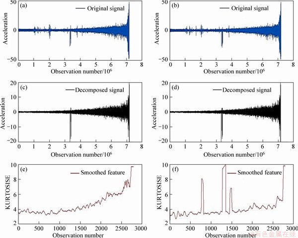
Figure 5 Main signal for vibrations of horizontal (a) and vertical (b), decomposed signal for vibration of horizontal (c) and vertical (d), extracted feature for vibration of horizontal (e) and vertical (f)
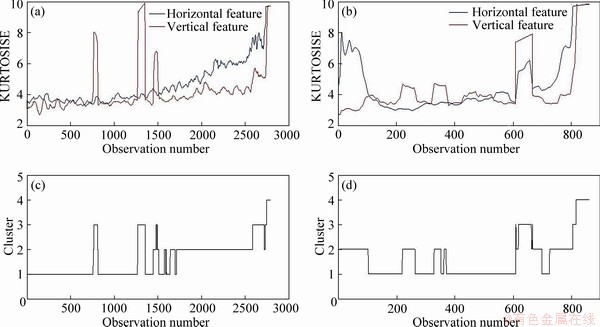
Figure 6 Vertical and horizontal features for bearing 1-1 (a) and bearing 1-2 (b), combing clusters for bearing 1-1 (c) and bearing 1-2 (d)
Table 4 FSR for learning bearings
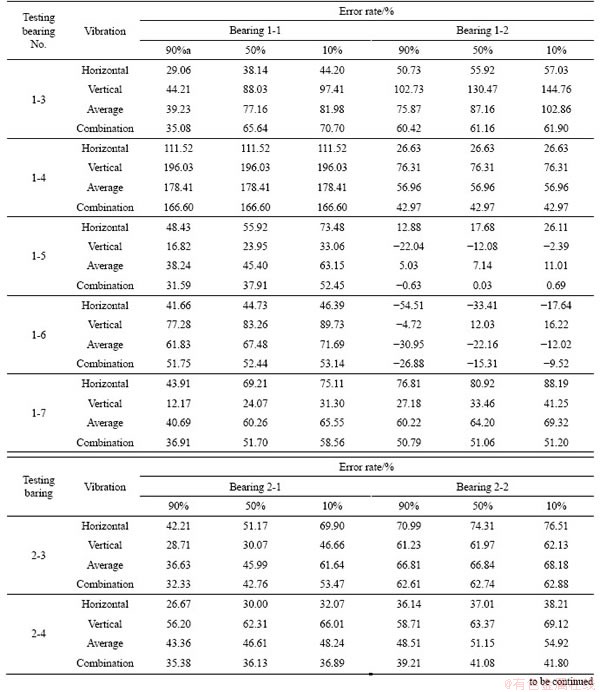
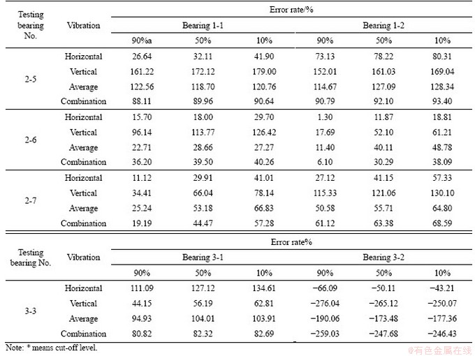
In Table 6, the forecasting error rate of the RUL of i-th bearing for each one of the cut-off levels is shown. The error rate is defined as follow:
 (27)
(27)
where ActRULi is the actual RUL and predRULi is hte predicted RUL of the i-th bearing.
Table 5 Determining lags of ARMRS model for learning bearings
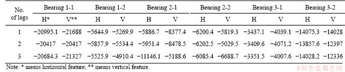
Table 6 Comparison of the combination approaches
Continued
Because in the process of determining the degradation state, bearing 1-4 has entered the final state, its RUL is calculated by considering  . As can be seen, in some bearings,there is a major difference in the estimation of the RUL by different learning bearings. In other words, the behavior of each of the testing bearings is more similar to one of the learning bearings. Comparing the error rates of the combination method and the only horizontal and only vertical sensors shows that the error rate in the combination method lies between those of the only horizontal and the only vertical sensors. In the absence of knowledge about the equipment physics of failure and the need to making decisions by different sensors, the use of the combination method can be helpful.
Considering 22 forecasting (10 cases for conditions 1, 10 cases for conditions 2 and 2 cases for conditions 3), in 20 out of 22 cases, the proposed combination method showed a better performance, in comparison with to the averaging method. Figure 7 shows the results of this comparison.
4.4 Comparing forecasting methods
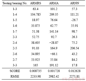
In order to evaluate the ARMRS forecasting method, its results are compared with two autoregressive forecasting methods: autoregressive moving average (ARMA) and autoregressive neural network by considering two criteria, SCORE [83] and RMSE:
 (28)
(28)
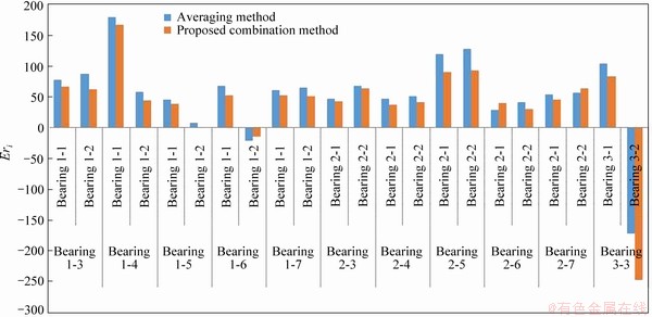
Figure 7 Comparison of results of averaging method and proposed combination method
 (29)
(29)
 (30)
(30)
The SCORE criterion allocates more penalties to overestimated forecasting.
The process of determining the parameters of autoregressive (AR) and moving average (MA) terms in the ARMA model is similar to that of the ARMRS model in the testing phase. Also, in this phase, the ARNN model is trained for each of the learning bearings. The learning rate, number of hidden layers and number of neurons in each of the hidden layers are tuned based on the two learning bearings. In Table 7, the results of the comparison between these three methods are shown. For each testing bearing, the average error rate in 50% cut-of level is calculated according to the two learning bearings and is considered as the final error rate. This error rate is calculated for each of the forecasting methods and is shown in the row for each of the testing bearings. As shown in Table 7, the ARNN performs better based on the SCORE criterion while the ARMRS performs better based on the RMSE criterion. In other words, the prediction accuracy of the ARMRS method was better considering the symmetry in prediction error.
Table 7 Comparison of forecasting methods
5 Conclusions
In this study, a condition monitoring model for determining the degradation states and estimating the RUL of a rotating equipment was presented. In this model, an autoregressive Markov regime switching was used for forecasting and simulation. In addition, a combination of the fuzzy c-mean clustering and the Dempster-Shafer theory was employed for determining the degradation state. In the proposed method for combining the sensor information, each sensor was considered as an evidence source. The probability that the system will be assigned to each fault state was calculated based on the equipment HI distance from the predetermined cluster center which was obtained by fuzzy c-means algorithm. Additionally, a new vibration-based feature, KURTOSISE, was introduced to represent the process of health/ degradation. In order to evaluate the model, the FEMTO-ST Institute��s dataset has been used. The proposed combination method can be used in situations where information about the physics of failure does not exist and decision making about the degradation state can be misleading considering the separate information of the sensors. The results of the proposed method of this study have shown its better performance than the averaging data combination method. Also, the autoregressive Markov regime switching (ARMRS) forecasting method can provide a proper performance in forecasting situations when there is a change in the states. By considering the symmetry in forecasting error, the forecasting performance of this method is better than the competing methods: autoregressive moving average (ARMA) and autoregressive neural network (ARNN).
Appendix A
Monotonicity represents the underlying increasing or decreasing trend of a time series and is calculated by the following equation:
 (31)
(31)
where m is the number of observations. The value of  can be from 0 to 1. Highly monotonic HI has =1 while the most non-monotonic HI has =0.
Trendability is related to the correlation between a data series with time and shows how the HI state varies with time. This criterion is calculated by the following equation:
 (32)
(32)
In this study, using the learning data of the case study (6 bearings), the average values of these criteria were calculated for two HIs.
References
[1] LEE J, WU F J, ZHAO W, GHAFFARI M, LIAO L X, SIEGEL D. Prognostics and health management design for rotary machinery systems: Reviews, methodology and applications [J]. Mechanical Systems and Signal Processing, 2014, 42(1, 2): 314-334. DOI: 10.1016/j.ymssp.2013. 06.004.
[2] TAHAN M, TSOUTSANIS E, MUHAMMAD M, ABDUL KARIM Z A. Performance-based health monitoring, diagnostics and prognostics for condition-based maintenance of gas turbines: A review [J]. Applied Energy, 2017, 198: 122-144. DOI: 10.1016/j.apenergy.2017.04.048.
[3] KAN M S, TAN A C C, MATHEW J. A review on prognostic techniques for non-stationary and non-linear rotating systems [J]. Mechanical Systems and Signal Processing, 2015, 62-63: 1-20. DOI: 10.1016/j.ymssp.2015.02.016.
[4] AN D, KIM N H, CHOI J H. Practical options for selecting data-driven or physics-based prognostics algorithms with reviews [J]. Reliability Engineering & System Safety, 2015, 133: 223-236. DOI: 10.1016/j.ress.2014.09.014.
[5] RAI A, UPADHYAY S H. A review on signal processing techniques utilized in the fault diagnosis of rolling element bearings [J]. Tribology International, 2016, 96: 289-306. DOI: 10.1016/j.triboint.2015.12.037.
[6] MOSALLAM A, MEDJAHER K, ZERHOUNI N. Data- driven prognostic method based on Bayesian approaches for direct remaining useful life prediction [J]. Journal of Intelligent Manufacturing, 2016, 27(5): 1037-1048. DOI: 10.1007/s10845-014-0933-4.
[7] DENG Y J, BARROS A, GRALL A. Degradation modeling based on a time-dependent Ornstein-Uhlenbeck process and residual useful lifetime estimation [J]. IEEE Transactions on Reliability, 2016, 65(1): 126-140. DOI: 10.1109/TR.2015. 2462353.
[8] REN Lei, CUI Jin, SUN Ya-qiang, CHENG Xue-jun. Multi-bearing remaining useful life collaborative prediction: A deep learning approach [J]. Journal of Manufacturing Systems, 2017, 43: 248-256. DOI: 10.1016/j.jmsy.2017. 02.013.
[9] SUTRISNO E, OH H, VASAN A S S, PECHT M. Estimation of remaining useful life of ball bearings using data driven methodologies [C]// 2012 IEEE Conference on Prognostics and Health Management. Denver. New York, USA: IEEE, 2012. DOI: 10.1109/ICPHM.2012.6299548.
[10] KIMOTHO J K, SONDERMANN-WOELKE C, MEYER T, SEXTRO W. Machinery prognostic method based on multi-class support vector machines and hybrid differential evolution-particle swarm optimization [J]. Chemical Engineering Transactions, 2013, 33: 619-624. DOI: 10.3303/ CET1333104.
[11] HONG Sheng, ZHOU Zheng, ZIO E, WANG Wen-bin. An adaptive method for health trend prediction of rotating bearings [J]. Digital Signal Processing, 2014, 35: 117-123. DOI: 10.1016/j.dsp.2014.08.006.
[12] HONG S, ZHOU Z, ZIO E, HONG K. Condition assessment for the performance degradation of bearing based on a combinatorial feature extraction method [J]. Digital Signal Processing, 2014, 27: 159-166. DOI: 10.1016/j.dsp.2013. 12.010.
[13] ZURITA D, CARINO J A, DELGADO M, ORTEGA J A. Distributed neuro-fuzzy feature forecasting approach for condition monitoring [C]// Proceedings of the 2014 IEEE Emerging Technology and Factory Automation (ETFA). New York, USA: IEEE, 2014. DOI: 10.1109/ETFA.2014.7005180.
[14] SOUALHI A, MEDJAHER K, ZERHOUNI N. Bearing health monitoring based on Hilbert�CHuang transform, support vector machine, and regression [J]. IEEE Transactions on Instrumentation and Measurement, 2015, 64(1): 52-62. DOI: 10.1109/TIM.2014.2330494.
[15] NIE Yu-ting, WAN Jiu-qing. Estimation of remaining useful life of bearings using sparse representation method [C]// 2015 Prognostics and System Health Management Conference (PHM). New York, USA: IEEE, 2015. DOI: 10.1109/PHM.2015.7380094.
[16] ZHANG Bin, ZHANG Li-jun, XU Jin-wu. Degradation feature selection for remaining useful life prediction of rolling element bearings [J]. Quality and Reliability Engineering International, 2016, 32(2): 547-554. DOI: 10.1002/qre.1771.
[17] GUO Liang, GAO Hong-li, HUANG Hai-feng, HE Xiang, LI Shi-chao. Multifeatures fusion and nonlinear dimension reduction for intelligent bearing condition monitoring [J]. Shock and Vibration, 2016: 1-10. DOI: 10.1155/2016/ 4632562.
[18] MOSALLAM A, MEDJAHER K, ZERHOUNI N. Time series trending for condition assessment and prognostics [J]. Journal of Manufacturing Technology Management, 2014, 25(4): 550-567. DOI: 10.1108/JMTM-04-2013-0037.
[19] LI Nai-peng, LEI Ya-guo, LIN Jing, DING S X. An improved exponential model for predicting remaining useful life of rolling element bearings [J]. IEEE Transactions on Industrial Electronics, 2015, 62(12): 7762-7773. DOI: 10.1109/TIE.2015.2455055.
[20] WANG Lu, ZHANG Li, WANG Xue-zhi. Reliability estimation and remaining useful lifetime prediction for bearing based on proportional hazard model [J]. Journal of Central South University, 2015, 22(12): 4625-4633. DOI: 10.1007/s11771-015-3013-9.
[21] CARINO J A, ZURITA D, DELGADO M, ORTEGA J A, ROMERO-TRONCOSO R J. Remaining useful life estimation of ball bearings by means of monotonic score calibration [C]// 2015 IEEE International Conference on Industrial Technology (ICIT). New York, USA: IEEE, 2015. DOI: 10.1109/ICIT.2015.7125351.
[22] LEI Ya-guo, LI Nai-peng, LIN Jing. A new method based on stochastic process models for machine remaining useful life prediction [J]. IEEE Transactions on Instrumentation and Measurement, 2016, 65(12): 2671-2684. DOI: 10.1109/ TIM.2016.2601004.
[23] NIU G, QIAN F, CHOI B K. Bearing life prognosis based on monotonic feature selection and similarity modeling [J]. Proceedings of the Institution of Mechanical Engineers, Part C: Journal of Mechanical Engineering Science, 2016, 230(18): 3183-3193. DOI: 10.1177/0954406215608892.
[24] HUANG Ze-yi, XU Zheng-guo, KE Xiao-jie, WANG Wen-hai, SUN You-xian. Remaining useful life prediction for an adaptive skew-Wiener process model [J]. Mechanical Systems and Signal Processing, 2017, 87: 294-306. DOI: 10.1016/j.ymssp.2016.10.027.
[25] CHENG Zhi-wei. Residual useful life prediction for rolling element bearings based on multi-feature fusion regression [C]// 2017 International Conference on Sensing, Diagnostics, Prognostics, and Control (SDPC). New York, USA: IEEE, 2017. DOI: 10.1109/SDPC.2017.54.
[26] TRINH H C, KWON Y K. An empirical investigation on a multiple filters-based approach for remaining useful life prediction [J]. Machines, 2018, 6(3): 35. DOI: 10.3390/ machines6030035.
[27] REN Lei, SUN Ya-qiang, CUI Jin, ZHANG Lin. Bearing remaining useful life prediction based on deep autoencoder and deep neural networks [J]. Journal of Manufacturing Systems, 2018, 48: 71-77. DOI: 10.1016/j.jmsy.2018. 04.008.
[28] REN Lei, SUN Ya-qiang, WANG Hao, ZHANG Lin. Prediction of bearing remaining useful life with deep convolution neural network [J]. IEEE Access, 2018, 6: 13041-13049. DOI: 10.1109/ACCESS.2018.2804930.
[29] DENG Sheng-cai, CHEN Zhi-qiang, CHEN Zhuo. Auxiliary particle filter-based remaining useful life prediction of rolling bearing [C]// 2017 International Conference on Sensing, Diagnostics, Prognostics, and Control (SDPC). New York, USA: IEEE, 2017. DOI: 10.1109/SDPC.2017.13.
[30] WU Yu-ting, YUAN Mei, DONG Shao-peng, LIN Li, LIU Ying-qi. Remaining useful life estimation of engineered systems using vanilla LSTM neural networks [J]. Neurocomputing, 2018, 275: 167-179. DOI: 10.1016/ j.neucom.2017.05.063.
[31] LI Xiang, ZHANG Wei, DING Qian. Deep learning-based remaining useful life estimation of bearings using multi-scale feature extraction [J]. Reliability Engineering & System Safety, 2019, 182: 208-218. DOI: 10.1016/j.ress.2018. 11.011.
[32] BEN ALI J, CHEBEL-MORELLO B, SAIDI L, MALINOWSKI S, FNAIECH F. Accurate bearing remaining useful life prediction based on Weibull distribution and artificial neural network [J]. Mechanical Systems and Signal Processing, 2015, 56-57: 150-172. DOI: 10.1016/j.ymssp. 2014.10.014.
[33] ZHAO Ming-hang, TANG Bao-ping, TAN Qian. Bearing remaining useful life estimation based on time�Cfrequency representation and supervised dimensionality reduction [J]. Measurement, 2016, 86: 41-55. DOI: 10.1016/ j.measurement.2015.11.047.
[34] LIAO Lin-xia, JIN Wen-jing, PAVEL R. Enhanced restricted boltzmann machine with prognosability regularization for prognostics and health assessment [J]. IEEE Transactions on Industrial Electronics, 2016, 63(11): 7076-7083. DOI: 10.1109/TIE.2016.2586442.
[35] WANG Zhao-qiang, HU Chang-hua, FAN Hong-dong. Real-time remaining useful life prediction for a nonlinear degrading system in service: application to bearing data [J]. ASME Transactions on Mechatronics, 2018, 23(1): 211-222. DOI: 10.1109/TMECH.2017.2666199.
[36] SINGLETON R K, STRANGAS E G, AVIYENTE S. Extended kalman filtering for remaining-useful-life estimation of bearings [J]. IEEE Transactions on Industrial Electronics, 2015, 62(3): 1781-1790. DOI: 10.1109/TIE. 2014.2336616.
[37] FENG Yang, HUANG Xiao-diao, HONG Rong-jing, CHEN Jie. Online residual useful life prediction of large-size slewing bearings: A data fusion method [J]. Journal of Central South University, 2017, 24(1): 114-126. DOI: 10.1007/s11771-017-3414-z.
[38] LIU Yu-mei, ZHAO Cong-cong, XIONG Ming-ye, ZHAO Ying-hui, QIAO Ning-guo, TIAN Guang-dong. Assessment of bearing performance degradation via extension and EEMD combined approach [J]. Journal of Central South University, 2017, 24(5): 1155-1163. DOI: 10.1007/s11771- 017-3518-5.
[39] BENKEDJOUH T, MEDJAHER K, ZERHOUNI N, RECHAK S. Remaining useful life estimation based on nonlinear feature reduction and support vector regression [J]. Engineering Applications of Artificial Intelligence, 2013, 26(7): 1751-1760. DOI: 10.1016/j.engappai.2013.02.006.
[40] LEI Ya-guo, LI Nai-peng, GONTARZ S, LIN Jing, RADKOWSKI S, DYBALA J. A model-based method for remaining useful life prediction of machinery [J]. IEEE Transactions on Reliability, 2016, 65(3): 1314-1326. DOI: 10.1109/TR.2016.2570568.
[41] LI Hong-kun, WANG Yin-hu. Rolling bearing reliability estimation based on logistic regression model [C]// 2013 International Conference on Quality, Reliability, Risk, Maintenance, and Safety Engineering (QR2MSE). New York, USA: IEEE, 2013. DOI: 10.1109/QR2MSE.2013.6625910.
[42] LI Yao-long, LI Hong-ru, WANG Bing, GU Hong-qiang. Rolling element bearing performance degradation assessment using variational mode decomposition and Gath- geva clustering time series segmentation [J]. International Journal of Rotating Machinery, 2017: 1-12. DOI: 10.1155/ 2017/2598169.
[43] SLOUKIA F, AROUSSI M E, MEDROMI H, WAHBI M. Bearings prognostic using mixture of gaussians hidden Markov model and support vector machine [C]// 2013 ACS International Conference on Computer Systems and Applications (AICCSA). New York, USA: IEEE, 2013. DOI: 10.1109/AICCSA.2013.6616438.
[44] WANG Yu, PENG Yi-zhen, ZI Yan-yang, JIN Xiao-hang, TSUI K L. A two-stage data-driven-based prognostic approach for bearing degradation problem [J]. IEEE Transactions on Industrial Informatics, 2016, 12(3): 924-932. DOI: 10.1109/TII.2016.2535368.
[45] MEDJAHER K, ZERHOUNI N, BAKLOUTI J. Data-driven prognostics based on health indicator construction: Application to PRONOSTIA��s data [C]// 2013 European Control Conference (ECC). New York, USA: IEEE, 2013. DOI: 10.23919/ECC.2013.6669223.
[46] LOUTAS T H, ROULIAS D, GEORGOULAS G. Remaining useful life estimation in rolling bearings utilizing data-driven probabilistic E-support vectors regression [J]. IEEE Transactions on Reliability, 2013, 62(4): 821-832. DOI: 10.1109/TR.2013.2285318.
[47] BOSKOSKI P, GASPERIN M, PETELIN D. Bearing fault prognostics based on signal complexity and Gaussian process models [C]// 2012 IEEE Conference on Prognostics and Health Management. New York, USA: IEEE, 2012. DOI: 10.1109/ICPHM.2012.6299545.
[48] WANG Tian-yi. Bearing life prediction based on vibration signals: A case study and lessons learned [C]// 2012 IEEE Conference on Prognostics and Health Management. New York, USA: IEEE, 2012. DOI: 10.1109/ICPHM.2012. 6299547.
[49] POROTSKY S. Remaining useful life estimation for systems with non-trendability behaviour [C]// 2012 IEEE Conference on Prognostics and Health Management. New York, USA: IEEE, 2012. DOI: 10.1109/ICPHM.2012.6299544.
[50] PAN Yong-ping, ER M J, LI Xiang, YU Hao-yong, GOURIVEAU R. Machine health condition prediction via online dynamic fuzzy neural networks [J]. Engineering Applications of Artificial Intelligence, 2014, 35: 105-113. DOI: 10.1016/j.engappai.2014.05.015.
[51] XIAO Lei, CHEN Xiao-hui, ZHANG Xing-hui, LIU Min. A novel approach for bearing remaining useful life estimation under neither failure nor suspension histories condition [J]. Journal of Intelligent Manufacturing, 2017, 28(8): 1893- 1914. DOI: 10.1007/s10845-015-1077-x.
[52] FUMEO E, ONETO L, ANGUITA D. Condition based maintenance in railway transportation systems based on big data streaming analysis [J]. Procedia Computer Science, 2015, 53: 437-446. DOI: 10.1016/j.procs.2015.07.321.
[53] JAVED K, GOURIVEAU R, ZERHOUNI N, NECTOUX P. Enabling health monitoring approach based on vibration data for accurate prognostics [J]. IEEE Transactions on Industrial Electronics, 2015, 62(1): 647-656. DOI: 10.1109/TIE. 2014.2327917.
[54] AN D, KIM N H, CHOI J. Bearing prognostics method based on entropy decrease at specific frequency [C]// 18th AIAA Non-Deterministic Approaches Conference. Reston, Virginia: AIAA, 2016. DOI: 10.2514/6.2016-1678.
[55] HINCHI A Z, TKIOUAT M. Rolling element bearing remaining useful life estimation based on a convolutional long-short-term memory network [J]. Procedia Computer Science, 2018, 127: 123-132. DOI: 10.1016/j.procs.2018. 01.106.
[56] JAVED K, GOURIVEAU R, ZERHOUNI N. Novel failure prognostics approach with dynamic thresholds for machine degradation [C]// IECON 2013-39th Annual Conference of the IEEE Industrial Electronics Society. New York, USA: IEEE, 2013. DOI: 10.1109/IECON.2013.6699844.
[57] KHADERSAB A, SHIVAKUMAR S. Vibration analysis techniques for rotating machinery and its effect on bearing faults [J]. Procedia Manufacturing, 2018, 20: 247-252. DOI: 10.1016/j.promfg.2018.02.036.
[58] SHAO Hai-dong, JIANG Hong-kai, LI Xing-qiu, LIANG Tian-chen. Rolling bearing fault detection using continuous deep belief network with locally linear embedding [J]. Computers in Industry, 2018, 96: 27-39. DOI: 10.1016/ j.compind.2018.01.005.
[59] SHE Dao-ming, JIA Min-ping. Wear indicator construction of rolling bearings based on multi-channel deep convolutional neural network with exponentially decaying learning rate [J]. Measurement, 2019, 135: 368-375. DOI: 10.1016/j.measurement.2018.11.040.
[60] PEARSON R K. Outliers in process modeling and identification [J]. IEEE Transactions on Control Systems Technology, 2002, 10(1): 55-63. DOI: 10.1109/87.974338.
[61] BABU C N, REDDY B E. A moving-average filter based hybrid ARIMA�CANN model for forecasting time series data [J]. Applied Soft Computing, 2014, 23: 27-38. DOI: 10.1016/j.asoc.2014.05.028.
[62] PAN Yu-na, CHEN Jin, LI Xing-lin. Bearing performance degradation assessment based on lifting wavelet packet decomposition and fuzzy c-means [J]. Mechanical Systems and Signal Processing, 2010, 24(2): 559-566. DOI: 10.1016/j.ymssp.2009.07.012.
[63] CHENG Chang-qing, SA-NGASOONGSONG A, BEYCA O, LE T, YANG Hui, KONG Z (, BUKKAPATNAM S T S. Time series forecasting for nonlinear and non-stationary processes: a review and comparative study [J]. IIE Transactions, 2015, 47(10): 1053-1071. DOI: 10.1080/ 0740817X.2014.999180.
[64] WANG Sheng-nan, ZHANG Xiao-yong, GAO Dian-zhu, CHEN Bin, CHENG Yi-jun, YANG Ying-ze, YU Wen-tao, HUANG Zhi-wu, PENG Jun. A remaining useful life prediction model based on hybrid long-short sequences for engines [C]// 2018 21st International Conference on Intelligent Transportation Systems (ITSC). New York, USA: IEEE, 2018. DOI: 10.1109/ITSC.2018.8569668.
[65] WANG Dong, ZHAO Yang, YANG Fang-fang, TSUI K L. Nonlinear-drifted Brownian motion with multiple hidden states for remaining useful life prediction of rechargeable batteries [J]. Mechanical Systems and Signal Processing, 2017, 93: 531-544. DOI: 10.1016/j.ymssp.2017.02.027.
[66] YAN Ji-hong, LEE J. A hybrid method for on-line performance assessment and life prediction in drilling operations [C]//2007 IEEE International Conference on Automation and Logistics. New York, USA: IEEE, 2007. DOI: 10.1109/ICAL.2007.4338999.
[67] PHAM H T, TRAN V T, YANG B S. A hybrid of nonlinear autoregressive model with exogenous input and autoregressive moving average model for long-term machine state forecasting [J]. Expert Systems with Applications, 2010, 37(4): 3310-3317. DOI: 10.1016/j.eswa.2009.10.020.
[68] WU Wei, HU Jing-tao, ZHANG Ji-long. Prognostics of machine health condition using an improved ARIMA-based prediction method [C]// 2007 2nd IEEE Conference on Industrial Electronics and Applications. New York, USA: IEEE, 2007. DOI: 10.1109/ICIEA.2007.4318571.
[69] ZHOU Yapeng, HUANG Miaohua. Lithium-ion batteries remaining useful life prediction based on a mixture of empirical mode decomposition and ARIMA model [J]. Microelectronics Reliability, 2016, 65: 265-273. DOI: 10.1016/j.microrel.2016.07.151.
[70] RAI A, UPADHYAY S H. The use of MD-CUMSUM and NARX neural network for anticipating the remaining useful life of bearings [J]. Measurement, 2017, 111: 397-410. DOI: 10.1016/j.measurement.2017.07.030.
[71] BEN ALI J, FNAIECH N, SAIDI L, CHEBEL-MORELLO B, FNAIECH F. Application of empirical mode decomposition and artificial neural network for automatic bearing fault diagnosis based on vibration signals [J]. Applied Acoustics, 2015, 89: 16-27. DOI: 10.1016/ j.apacoust.2014.08.016.
[72] SAMANTA B, AL-BALUSHI K R. Artificial neural network based fault diagnostics of rolling element bearings using time-domain features [J]. Mechanical Systems and Signal Processing, 2003, 17(2): 317-328. DOI: 10.1006/mssp. 2001.1462.
[73] ZHENG Xiu-juan, FANG Hua-jing. An integrated unscented kalman filter and relevance vector regression approach for lithium-ion battery remaining useful life and short-term capacity prediction [J]. Reliability Engineering & System Safety, 2015, 144: 74-82. DOI: 10.1016/j.ress.2015.07.013.
[74] ANDRE D, NUHIC A, SOCZKA-GUTH T, SAUER D U. Comparative study of a structured neural network and an extended Kalman filter for state of health determination of lithium-ion batteries in hybrid electricvehicles [J]. Engineering Applications of Artificial Intelligence, 2013, 26(3): 951-961. DOI: 10.1016/j.engappai.2012.09.013.
[75] HOCHSTEIN A, AHN H I, LEUNG Y T, DENESUK M. Switching vector autoregressive models with higher-order regime dynamics Application to prognostics and health management [C]// 2014 International Conference on Prognostics and Health Management. New York, USA: IEEE, 2014.
[76] PENG Yi-zhen, WANG Yu, ZI Yan-yang. Switching state-space degradation model with recursive filter/smoother for prognostics of remaining useful life [J]. IEEE Transactions on Industrial Informatics, 2019, 15(2): 822-832. DOI: 10.1109/TII.2018.2810284.
[77] HAMILTON J D. Regime switching models [M]. Macroeconometrics and Time Series Analysis. London, UK: Palgrave Macmillan UK, 2010: 202-209. DOI: 10.1057/ 9780230280830_23.
[78] SCHWARZ G. Estimating the dimension of a model [J]. The annals of statistics, 1978, 6(2): 461-464. https://projecteuclid. org/euclid.aos/1176344136.
[79] PERLIN M. MS_Regress-the MATLAB package for Markov regime switching models [R]. 2015. DOI: 10.2139/ssrn. 1714016.
[80] SHAFER G. A mathematical theory of evidence [M]. Princeton: Princeton University Press, 1976. https://press. princeton.edu/titles/2439.html.
[81] SENTZ K, FERSON S. Combination of evidence in Dempster-Shafer theory [R]. Office of Scientific and Technical Information (OSTI), 2002. DOI: 10.2172/800792.
[82] SMARANDACHE F, DEZERT J. Advances and applications of DSmT for information fusion [R]. Collected Works, 2015. https://hal.archives-ouvertes.fr/hal-01080187/.
[83] NECTOUX P, GOURIVEAU R, MEDJAHER K, RAMASSO E, CHEBEL-MORELLO B, ZERHOUNI N, VARNIER C. PRONOSTIA: An experimental platform for bearings accelerated degradation tests [C]// IEEE International Conference on Prognostics and Health Management. PHM��12. 2012: CPF12PHM-CDR. https://hal. archives-ouvertes.fr/hal-00719503.
(Edited by ZHENG Yu-tong)
���ĵ���
�����˻�״̬ȷ����ת�豸ʣ��ʹ��������ģ��
ժҪ��״̬�������豸������������Ҫ����֮һ��PHM����������CBM��һ�ַ�չ��ʽ����������������������Ҫ�IJ��衣���Ľ�ϴ�������Ϣ������״̬��ȷ���ͽ���ָ���Ԥ�⣬�������豸��ʣ��ʹ������������һ��ȷ��Demster-Shafer��Ϲ�����ʵ��·�����ģ��c��ֵ������Դ�������Ϣ������ϡ������Իع������ɷ�״̬ת��(ARMR)��������ȡ�Ļ����Ľ���ָ������ģ���Ԥ�⣬ȷ�����յĽ���״̬������ʣ������(RUL)��Ϊ�˶�ģ�ͽ������ۣ�ʹ����FEMTO-ST�о����ṩ�Ĵ��������ݡ�
�ؼ��ʣ�ʣ��ʹ��������Ԥ���뽡���������Իع������ɷ�״̬ת��������ָ��(HI); Dempster-Shafer���ۣ�ģ��c��ֵ����Kurtosis-entropy���˻�
Received date: 2018-11-09; Accepted date: 2019-07-04
Corresponding author: Alireza MOINI, PhD, Associate Professor; Tel: +98-2173225000; E-mail: moini@iust.ac.ir; ORCID: https:// orcid.org/0000-0002-0565-7744
Abstract: Condition assessment is one of the most significant techniques of the equipment��s health management. Also, in PHM methodology cycle, which is a developed form of CBM, condition assessment is the most important step of this cycle. In this paper, the remaining useful life of the equipment is calculated using the combination of sensor information, determination of degradation state and forecasting the proposed health index. The combination of sensor information has been carried out using a new approach to determining the probabilities in the Dempster-Shafer combination rules and fuzzy c-means clustering method. Using the simulation and forecasting of extracted vibration-based health index by autoregressive Markov regime switching (ARMRS) method, final health state is determined and the remaining useful life (RUL) is estimated. In order to evaluate the model, sensor data provided by FEMTO-ST Institute have been used.
