
J. Cent. South Univ. Technol. (2010) 17: 1300-1309
DOI: 10.1007/s11771-010-0635-9![]()
Assessment of grid inherent vulnerability considering open circuit fault under potential energy framework
LIU Qun-ying(��ȺӢ)1, LIU Qi-fang(����)2, HUANG Qi(����)1, LIU Jun-yong(������)3
1. School of Automation, University of Electronic Science and Technology, Chengdu 611731, China;
2. China Guodian Corporation, Sichuan Ashine Power Co. Ltd, Chengdu 610041, China;
3. School of Electrical Engineering and Information, Sichuan University, Chengdu 610065, China
? Central South University Press and Springer-Verlag Berlin Heidelberg 2010
Abstract:
A potential energy framework for assessment of grid vulnerability was presented. In the framework, the branch potential energy function model was constructed. Two indexes, current vulnerability and forecasting vulnerability, were calculated. The current vulnerability was used to identify the current vulnerable area through calculating the distance between the current transmitted power and initial transmitted power; and the forecast vulnerability under variation of power injection was used to predict the vulnerable area of next step and verify the current vulnerable area. Numerical simulation was performed under variant operating conditions with IEEE-30 bus system, which shows that almost area of 90% overlaps between current vulnerable area and forecasting vulnerable area, the overlapped area is termed as inherent vulnerable area of grid. When considering N-1 contingency, the assessment results of this method proposed agree with those of optimal power flow. When considering N-2 contingency, optimal power flow fails to obtain correct results, while the method based on energy framework gives reliable results.
Key words:
1 Introduction
The power system vulnerability has been a hot topic since its emergence, and attracts the attention of many researchers in power engineering. The technical approaches can be categorized as follows: (1) approach based on energy function; (2) approach based on probability and risk theory; (3) approach based on complex network theory; and (4) approach based on artificial intelligence.
FOUAD et al [1] and LIU et al [2] used energy margin and its variation trend with respect to the change in active power as the security index to assess system vulnerability. This method is widely used and can obtain results with certain degree of reliability.
Approach based on probability and risk theory is mainly used to assess the uncertainty of grid vulnerability. YU and SINGH [3] proposed optimal model of system relay, margin index and the security probability to assess system vulnerability. CHEN et al [4] proposed low voltage and over-load risk indexes to quantify the vulnerability.
With complex network theory, many influencing factors of grid [5-10] can be comprehensively considered when assessing the grid vulnerability. Based on complex network theory, CHEN et al [5] proposed the weighted branch betweenness to identify the branches that influence system vulnerability; CAO et al [6] used the grid connexity level as the criterion of system vulnerability; DING and HAN [7] proposed the impedance-based topological model and cascading failure model for weighted power grid, and the corresponding algorithm and new indices were established to calculate the average distance of weighted power grid; ZHANG et al [8] proposed the weighted and directional graph considering both the operational state and topological parameters; DING et al [9] presented a grid vulnerability analyzing method based on the two-dimensional accumulation means, in which, the modified small world network model was employed under given power system conditions; and BALDICK et al [10] used this theory to analyze cascading failures mechanism. The advantage of this method is that grid topological changes are considered to estimate system vulnerability.
Hoping to improve the computation velocity and considering the uncertainty factors of power system, HAIDAR et al [11], MINGOO et al [12] and INNOCENT et al [13] proposed artificial intelligence to assess grid vulnerability��but the results are not so good as expected. Besides, there are other methods such as index method [14] and clustering approach based on the fuzzy logic [15].
The unified definition of vulnerability is yet to be given [4, 7, 16]. In this work, the grid inherent vulnerability was defined as the characteristics of the sustained degrading of power transmission capability under disturbances or faults. According to previous analysis, these characteristics were found in different system operation modes. In this definition, LIU et al [2] proposed two indices to discuss the vulnerability of grid based on energy function. The assessment method based on energy function was further discussed to assess the inherent vulnerability in this work. First, branch potential energy (BPE) function model was constructed. Then, the maximal potential energy of every branch was calculated, and the current vulnerability index transformed from real power transmission state of the current branch was used to quantify the distance between the current state and stable state. With the combination of the current vulnerability and its developing trend, the forecast vulnerability index was proposed to predict the next possible vulnerable branch. The inherent vulnerable area of power grid was obtained as the overlapped vulnerability area of the assessment results from the two indices. Cases studies with IEEE-30 bus system were performed and the results were compared with those of optimal power flow considering N-1 and N-2 contingencies.
2 Construction of branch potential energy function model
2.1 BPE function model of two-bus system
The potential energy differences between nodes decide the branch power transmission. Of course, there are limits on branch power transmission, such as the thermal limit, voltage limit and economic factors. Accordingly, the branch potential energy is also limited. The branch power transmission includes real power and reactive power transmission. Their quantities are determined respectively by the phase angle difference and voltage amplitude difference. In the potential energy model, the real power transmission is integrated with phase angle difference, while the reactive power transmission is integrated with voltage amplitude difference. According to these relationships, the potential energy model of two-bus system can be established as Fig.1, where V1 represents the voltage amplitudes in node 1; V2 represents the voltage amplitudes in node 2; ��12=��1-��2, ��1 and ��2 represent the phase angles in node 1
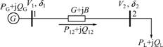
Fig.1 Schematic diagram of potential energy model of two-bus system
and node 2, respectively; P12 represents the real power transmission of some state in branch 12; Q12 represents the reactive power transmission of some state in branch 12; G represents the conductance in branch 12; B represents the susceptance in branch 12; PG and QG represent the real power and reactive power of operator; PL and GL represent the real power and reactive power of load.
In Fig.1, the relationship between V1 and V2 is expressed as
![]() (1)
(1)
where ![]() So there is
So there is
![]() (2)
(2)
Based on the relationship of branch power transmission, the power flow of branch 12 in Fig.1 is expressed as:
![]() (3)
(3)
![]() (4)
(4)
where fp12 and fq12 represent the function of P12 and Q12, respectively; ![]() represents initial stable value of P12 and
represents initial stable value of P12 and ![]() represents the initial stable value of Q12.
represents the initial stable value of Q12.
Based on the integral theory of energy [16], the branch potential energy function is expressed as follows:
![]()
![]()
![]()
![]() dV12(5)
dV12(5)
where ![]() and
and ![]() represent the initial stable voltage amplitudes, respectively,
represent the initial stable voltage amplitudes, respectively, ![]()
![]() and
and![]() represent the initial phase angles of ��1 and ��2, respectively,
represent the initial phase angles of ��1 and ��2, respectively, ![]()
On the premise of reactive power being adequate, the change of voltage amplitude is small. Accordingly, the potential energy generated by the reactive power in Eq.(5) is almost 0. So the branch potential energy function is expressed as:
![]() d��12=
d��12=
![]() (6)
(6)
According to Eq.(6), when P12 is equal to ![]() E12 is equal to 0. At this moment, the potential energy is the minimal. When P12 increases from
E12 is equal to 0. At this moment, the potential energy is the minimal. When P12 increases from ![]() forwardly or backwardly, |E12| will increase. However, when P12 reaches the limit of branch power transmission, |E12| will reach the limit of potential energy. When ��12 belongs
forwardly or backwardly, |E12| will increase. However, when P12 reaches the limit of branch power transmission, |E12| will reach the limit of potential energy. When ��12 belongs
to ![]() |E12| decreases firstly and then
|E12| decreases firstly and then
increases with the phase angles increasing. Actually, when ��12 changes along the direction ��12��![]() or ��12��
or ��12��![]() , |E12| will increase. When ��12 approaches to
, |E12| will increase. When ��12 approaches to ![]() , |E12| will decrease and approach to the minimal value (0).
, |E12| will decrease and approach to the minimal value (0).
2.2 BPE function model of multi-bus system
Based on the integral theory of energy and the analysis of two-bus system in section 2.1, the branch potential energy function of multi-bus system is expressed as
![]() (7)
(7)
where
![]()
![]() (8)
(8)
![]()
![]() (9)
(9)
where fpij and fqij represent the functions of Pij and Qij; Vi and Vj represent the voltage amplitudes in nodes i and j, respectively; ![]() and
and ![]() represent the initial voltage amplitudes in nodes i and j, respectively; Vij=Vi-Vj=
represent the initial voltage amplitudes in nodes i and j, respectively; Vij=Vi-Vj=
![]()
![]() represents the initial
represents the initial
stable voltage difference, ![]() ��i represents the phase angles in node i; ��j represents the phase angles in node j, ��ij=��i-��j, its initial stable phase angle difference is
��i represents the phase angles in node i; ��j represents the phase angles in node j, ��ij=��i-��j, its initial stable phase angle difference is ![]() ��j represents the load power
��j represents the load power
angle,![]() Pij represents the real power
Pij represents the real power
transmission in branch ij; ![]() represents its initial stable value; Qij represents the current reactive power transmission in branch ij;
represents its initial stable value; Qij represents the current reactive power transmission in branch ij; ![]() represents its initial stable value; Gij represents the conductance in branch ij; and Bij represents the susceptance of branch ij.
represents its initial stable value; Gij represents the conductance in branch ij; and Bij represents the susceptance of branch ij.
3 Construction of vulnerability assessment index
3.1 Current vulnerability
In Eq.(7), the integration of phase angle difference and voltage amplitude difference do not depend on the integral path, thus the energy is expressed as:
![]() (10)
(10)
Eqij corresponds to the potential energy of reactive power part. Assuming that the reactive power transmission is invariable during the period of real power transmission and the voltage amplitude changes little (namely, Eqij��0), the energy is
![]() (11)
(11)
where ��Pij=Pij-![]() With the full decoupling of P and Q, real power transmission can be expressed as:
With the full decoupling of P and Q, real power transmission can be expressed as:
![]() (12)
(12)
Compared with the initial power flow, the change of real power transmission in branch ij is:
![]() (13)
(13)
Substituting Eq.(13) to Eq.(11), the relationship between the potential energy and the change of real power transmission in branch ij is expressed as follows:
![]() (14)
(14)
Eq.(14) indicates that Pij shifts further from ![]() the absolute value of Eij is bigger. When Pij reaches
the absolute value of Eij is bigger. When Pij reaches ![]() the phase angle difference reaches
the phase angle difference reaches ![]() and Eij approaches
and Eij approaches ![]()
![]() represent the maximum of Pij, ��ij and Eij, respectively. Thus, based on the definition to system vulnerability, the current vulnerability of branch is proposed as follows:
represent the maximum of Pij, ��ij and Eij, respectively. Thus, based on the definition to system vulnerability, the current vulnerability of branch is proposed as follows:
 (15)
(15)
Based on Eq.(7), ![]() is shown as
is shown as
![]() (16)
(16)
where ![]() and
and ![]() are the upper limit and lower limit of phase angle difference;
are the upper limit and lower limit of phase angle difference;![]() and
and![]() are the upper limit and lower limit of voltage amplitude difference. When reactive power of system is adequate, the potential energy of reactive power is almost 0. According to the physical meanings of vulnerability index, the qualitative conclusions are shown as follows:
are the upper limit and lower limit of voltage amplitude difference. When reactive power of system is adequate, the potential energy of reactive power is almost 0. According to the physical meanings of vulnerability index, the qualitative conclusions are shown as follows:
 (17)
(17)
According to Eq.(15), when 0��Iij��1, the branch transmission value lies in the system limit; when Ii =1, ![]() and the branch power transmitted reaches the limit borderline; when Iij��1, the branch power is out of limit. In conclusion, the advantage of Iij as vulnerability assessment index is that it can quantify the transmission state of branch power. At the same time, impacts from the voltage and phase angle are considered.
and the branch power transmitted reaches the limit borderline; when Iij��1, the branch power is out of limit. In conclusion, the advantage of Iij as vulnerability assessment index is that it can quantify the transmission state of branch power. At the same time, impacts from the voltage and phase angle are considered.
3.2 Forecasting vulnerability under impact of power injection change
Current vulnerability can give the distance information of the current state to stable borderline, but cannot forecast the next state change. The forecasting vulnerability, which can respond to the change of the power injection space, will compensate the shortcoming. With the full decoupling of P and Q, ��P=Jp-������, there is:
![]() (18)
(18)
where ���� represents the change of phase angle; ![]() represents Jacobian matrix corresponding to real power change. According to the branch power transmission equation, the change of the real power flow is shown as:
represents Jacobian matrix corresponding to real power change. According to the branch power transmission equation, the change of the real power flow is shown as:
![]() (19)
(19)
where ��i and ��j represent the change of phase angle at nodes i and j, respectively.
Substituting Eq.(18) into Eq.(19) , there is:
![]() (20)
(20)
where![]() Zi and Zj are respectively the
Zi and Zj are respectively the
elements of the ith and jth row. Assuming DIij=Eij/![]() DIij quantifies the degree of the current potential energy shifting from the stable state. It is expressed as:
DIij quantifies the degree of the current potential energy shifting from the stable state. It is expressed as:
![]() (21)
(21)
The differential coefficient of potential energy to power transmission in branch ij is expressed as follows:
![]() (22)
(22)
According to Eqs.(21) and (22), the change of DIij under the impacts of node power injection is expressed as:
![]()
 (23)
(23)
Thus, the forecasting vulnerability of branch is expressed as:
 (24)
(24)
where FIij,k+1 is the forecasting vulnerability with the impacts of the current power injection changing. The more the value of FIij,k+1 is, the more vulnerable the branch ij. By this index, the vulnerability change of the next step will be forecasted from the global system. The inherent vulnerable area will be got among the assessment results of the current vulnerability and the forecasting vulnerability. During the process of computation, only the Jacobian matrix corresponding to real power part is needed, so the computation is less than that of the traditional power flow computation.
Voltage amplitude and phase angle are involved in Eq.(24). Considering that this research was carried on by assuming reactive power being adequate, voltage amplitude is treated as constant and the limit of phase angle difference is derived from the initial states of system.
4 Algorithm process
Step 1 Construct the index model of branch vulnerability.
Step 2 Calculate the current vulnerability under the different system cases, and then sequence the results from high to low.
Step 3 Calculate the forecasting vulnerability under different systems as step 2.
Step 4 Judge the correctness of step 2 by comparing with the results of steps 2 and 3, and then determine the vulnerable area under the cases with the same property.
Step 5 Determine the inherent vulnerable branches under the cases with different properties according to the assessment results of step 4.
5 Example
Simulation system: IEEE-30 bus system with 6 generators respectively distributed in nodes 1 (slack node), 2, 5, 8, 11 and 13. Three kinds of system cases: Base case (e.g. the output of all generators increase and the requirements of all the load nodes increase), N-1 faults and N-2 faults. All the initial values were obtained by power flow computation. All the computation results were expressed as per-unit value with the base power 100 MW and base voltage 110 kV. Table 1 shows the relationship between the abscissa dots and the relative branches in the following simulation figures.
5.1 System vulnerability analysis under base case
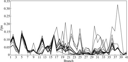
When the productions of generators 2, 11 and 13 respectively increase to 50 MW and all loads respectively increase to 50 MW, the current vulnerability curves are analyzed. Part of the simulation figures are shown as Figs.2-4, where I represents the current vulnerability index; pu represents per-unit value and the every curve represents the change of current vulnerability of all branches under different system cases.
According to the comparisons of Figs.2-4, when all load requirements respectively increase to the same level, branches 1-3, 2-5, 2-6, 6-10, 4-12, 10-20 and 28-27 show relatively high vulnerability, corresponding to the power injection of different generators. With the productions of all generators reaching the same level and all the load requirements increasing to the same level, the impacts from different generators on grid vulnerability are different. In Fig.2, with the production of generator 2 increasing, branches 1-2, 2-5, 2-6 and 2-4, which are directly linked with node 2, show relatively high vulnerability. At the same time, branches 1-3, 2-6, 6-10, 4-12 and 28-27 show strong vulnerable trend corresponding to the increase of load requirements. In Fig.3, compared with Fig.2, when the production of generator 11 increases, the power flow along branch 9-11 increases. So, its vulnerability increases. Meanwhile, branches 1-3, 2-5 and 4-12 show relatively high vulnerabilities, corresponding to the increase of load requirements. In Fig.4, when the production of generator 13 increases, the power flow along branch 12-13 increases by comparing with Fig.3. So, its vulnerability increases. Meanwhile, branch 1-3, 2-5, 6-10 and 4-12 show high vulnerabilities and branches 28-27 and 10-20 show weak vulnerabilities corresponding to the increase of load requirements. Compared with Fig.3, the vulnerabilities of branches 1-3, 4-12, 9-11 in Fig.4 are lower. But the vulnerability of branch 12-13 increases. However, when the requirements of different load nodes increase to the same level, the vulnerability of the nearest or the most correlative branches changes much. For example, the loads in nodes 26 and 30 are increased, the nearby branches 27-29, 27-30, 29-30 and 28-27 show high vulnerability. The transmission capabilities of branches 27-30, 27-29, 28-27, 25-27 and 24-25 are less than those of the other ones. So, when the requirements of the neighboring nodes increase to the same level as the other nodes, these branches will show high vulnerabilities, which does not mean that these branches are easy to be vulnerable within system wide and the same phenomenon will appear in the following simulations. The analysis about forecasting vulnerability is the same as the current vulnerability, so the simulations about it are omitted. The current vulnerable branches and the forecasting branches are shown in Table 2.
Table 1 Relationship between abscissa dots and branches
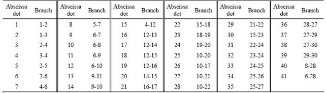
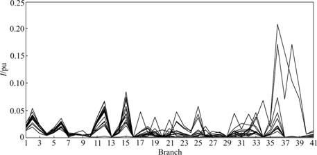
Fig.2 Overlapped I curves of system with increase of real power production of generator 2
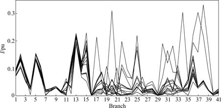
Fig.3 Overlapped I curves of system with increase of real power production of generator 11
Fg.4 Overlapped I curves of system with increase of real power production of generator 13
Table 2 Assessment results of current vulnerability and forecasting vulnerability
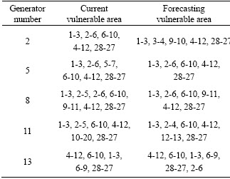
According to Table 2, the production of different generators and the increase of different loads will result in different branches to become vulnerable. However, the vulnerabilities of these branches that are near to generators will be decreased with the increase of the generators production, but the vulnerabilities of these branches, which are far from generators, will be increased. The simulation results of multiple cases of system indicate that there are always several branches that show high vulnerability to arbitrary power injection, such as branches 1-3, 2-6, 6-9, 6-10, 4-12 and 28-27. They are the overlapped branches between the current vulnerable area and the forecasting vulnerable area. In fact, these branches are the inherent vulnerable area of grid.
5.2 Vulnerability analysis under N-1 contingency
The curves of current vulnerability with branches 1-2 and 18-19 tripped are shown in Figs.5 and 6, respectively.
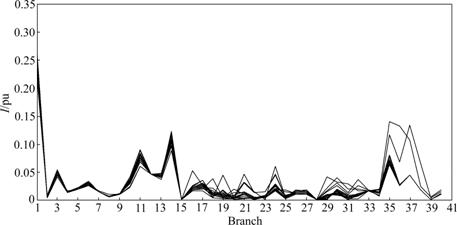
Fig.5 Overlapped I curves of system with branch 1-2 tripped
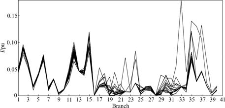
Fig.6 Overlapped I curves of system with branch 18-19 tripped
According to Figs.5 and 6, different power shifts will be caused by different tripped branches, so that the branch vulnerability will accordingly change. But branches 1-3, 2-6, 6-10 and 4-12 show high vulnerability to different power injections under N-1 faults. In Fig.5, branch 1-3 takes on the part of the task of branch 1-2, so its vulnerability increases. In Fig.6, the requirements in nodes 18 and 19 are increased, the real power along branch 18-19 is respectively shared by branches 12-15, 15-18, 19-20 and 10-20. Therefore, the vulnerabilities of these branches are changed greatly. At last, when the requirements of different load nodes are increased to the same level, the other assessment results with branches 1-3, 2-4, 3-4 and 2-5 being tripped are done, respectively.
According to the simulation results from N-1 contingency, the grid vulnerable area mainly concentrates in branches 1-3, 2-4, 2-5, 2-6, 6-10, 4-12 and 28-27. However, branches 6-10 and 4-12 show high vulnerability to all cases. As a result, much attention should be paid to them. However, tripping the two branches will cause in new vulnerable area. For example, when branch 6-10 is tripped, vulnerable branch will be changed from branch 6-10 to branch 6-9, and the inherent vulnerable area includes branches 1-3, 2-6, 6-9, 4-12 and 28-27; when branch 4-12 is tripped, the power flows in branch 6-10 and branch 28-27 will be increased and the inherent vulnerable area concentrates in branches 1-3, 2-6, 6-10, 9-10 and 28-27. Additionally, the conclusion can also be drawn that the inherent vulnerable area determined by the forecasting vulnerability is consistent with the current vulnerable area.
5.3 Vulnerability analysis under N-2 contingency
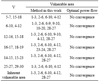
The I curves with branches 14-15, 15-23 and 25-27, 29-30 being tripped are shown in Figs.7 and 8, respectively.
According to Figs.7 and 8, the grid vulnerabilities under N-2 contingencies increase much more than those under N-1 contingencies. In Fig.7, with branches 14-15 and 15-23 being tripped and load in node 23 being increased, the vulnerabilities of branches 22-24, 24-25 and 25-27 are increased because of the share to the task of the branch 15-23. However, when the requirements in nodes 26, 29 and 30 increase, the vulnerabilities of branches nearby 28-27, 27-29, 27-30, 22-24 and 24-25 are increased. Current vulnerabilities of parts of them, such as branches 25-26, 28-27 and 27-30, exceed 1.0 and their power flows overflow. In Fig.8, when branches 25-27 and 29-30 are tripped, comparing with Fig.7, the vulnerabilities system-wide become worsen. The vulnerabilities of branches 27-30, 27-29, 28-27, 24-25 and 8-28 increase much with increase of the requirements in nodes 26, 29 and 30 and some even approach 1.4. This phenomenon shows that the power flows in these branches with serious overflow.
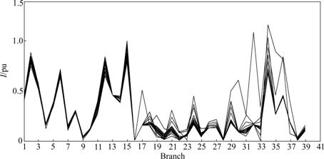
Fig.7 Overlapped I curves of system with branch 14-15 and 15-23 tripped
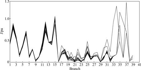
Fig.8 Overlapped I curves of system with branch 25-27 and 29-30 tripped
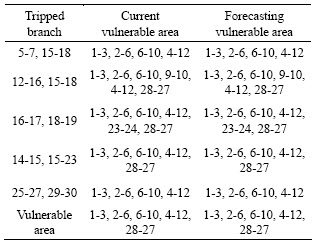
The assessment results of other branches being tripped are shown in Table 3. According to the simulations of N-2 contingencies, the conclusions can be drawn that the inherent vulnerable area from the current vulnerable area and the forecasting area are almost the same. Branches 1-3, 2-6, 6-10, 4-12 and 28-27 show high vulnerable trend corresponding to different load requirements at the same level. Thus, much attention should be paid to these branches during the system operation.
5.4 Synthetical analysis of inherent vulnerability under base case, N-1 contingency and N-2 contingency
According to the analysis above, although the assessment results of the specific cases are different, there is the same inherent vulnerable area among the same property cases. Among the base cases of system, the inherent vulnerable area consists of branches 1-3, 2-4, 2-5, 2-6, 6-10, 4-12, 10-20 and 28-27; among N-1 contingencies, the inherent vulnerable area consists of branches 1-3, 2-4, 2-5, 2-6, 6-10 and 4-12; among N-2 contingencies, the inherent vulnerable area consists of branches 1-3, 2-6, 6-10 and 4-12. The relationships among three different properties cases are shown in Fig.9.
Table 3 Comparison of assessment results of system vulnerability under N-2 contingencies
5.5 Comparison with optimal power flow computation
Comparisons between the method proposed in this work and the method of optimal power flow are listed in Tables 4 and 5.
According to the comparisons between Tables 4 and 5, under the same operation conditions, the results of two methods are almost the same, but the method proposed in this work shows more evident trend to the vulnerable branches, so the inherent vulnerable branch is easier to come out. In Table 5, because of the restriction of power flow convergence, the optimal power flow is powerless to the vulnerability assessment under N-2 contingencies. However, because of the advantages of catching the distribution state of grid vulnerability and the immunity to the restriction of power flow convergence, the method proposed in this work also attains the assessment results of grid inherent vulnerability under N-2 contingencies.
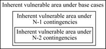
Fig.9 Assessment results comparison among three system cases
Table 4 Comparison of assessment results under N-1 contingencies between method proposed in this work and method of optimal power flow
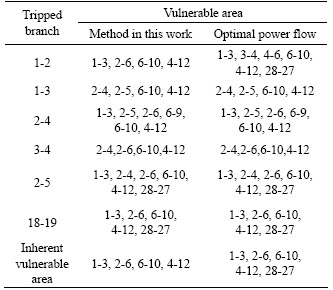
Table 5 Comparison of assessment results under N-2 contingencies between method proposed in this work and method of optimal power flow
6 Conclusions
(1) The assessment indexes of grid vulnerability based on branch potential energy can quantitatively and qualitatively assess the vulnerability of grid, and can be used to calculate the inherent vulnerable area.
(2) When considering N-1 and N-2 contingencies, the proposed indexes can avoid the limit of convergence problem in power flow, and can be used to analyze the variation profile of vulnerability.
(3) The high efficiency in computation with energy function may enhance its applicability to grid vulnerability assessment.
(4) The accuracy of phase angle difference of branch has significant impact on the correctness of the assessment results. The more accurate the phase-angle difference is, the more correct the assessment results are.
References
[1] FOUAD A A, QIN Z, VITTAL V. System vulnerability as a concept to assess power system dynamic security [J]. IEEE Transactions on Power Systems, 1994, 9(2): 1009-1015.
[2] LIU Qun-ying, LIU Jun-yong, LIU Qi-fang. Power grid vulnerability assessment based on branch potential energy information [J]. Automation of Electric Power Systems, 2008, 32(10): 6-11. (in Chinese)
[3] YU X B, SINGH C. A practical approach for integrated power system vulnerability analysis with protection failures [J]. IEEE Transactions on Power Systems, 2004, 19(4): 1811-1820.
[4] CHEN Wei-hua, JIANG Quan-yuan, CAO Yi-jia. HVDC system vulnerability assessment based on models combination and risk theory [J]. Automation of Electric Power System, 2005, 29(21): 19-24. (in Chinese)
[5] CHEN Xiao-gang, SUN Ke, CAO Yi-jia. Structural vulnerability analysis of large power grid based on complex network theory [J]. Transactions of China Eelectrotechnical Society, 2007, 22(10): 138-144. (in Chinese)
[6] CAO Yi-jia, CHEN Xiao-ming, SUN Ke. Identification of vulnerable lines in power grid based on complex network theory [J]. Electric Power Automation Equipment, 2006, 26(12): 1-5. (in Chinese)
[7] DING Ming, HAN Ping-ping. Vulnerability assessment to small-world power grid based on weighted topological model [J]. Automation of Electric Power System, 2008, 28(10): 20-25. (in Chinese)
[8] ZHANG Guo-hua, WANG Ce, ZHANG Jian-hua, YANG Jing-yan. Vulnerability assessment of bulk power grid based on complex network theory [C]// Proceedings of the Third International Conference on Electric Utility Deregulation and Restructuring and Power Technologies. Nanjing: IEEE Computer Society, 2008: 1554-1558.
[9] DING Jian, BAI Xiao-min, ZHAO Wei, LI Zai-hua. Grid vulnerability analysis based on two-dimensional accumulation means [J]. Automation of Electric Power Systems, 2008, 32(8): 1-4. (in Chinese)
[10] BALDICK R, CHOWDHURY B, DOBSON I. Vulnerability assessment for cascading failures in electric power systems [C]// Proceedings of Power Systems Conference and Exposition. Seattle: IEEE Computer Society, 2009: 1-9.
[11] HAIDAR A M A, MOHAMED A, HUSSAIN A. Vulnerability assessment of a large sized power system using radial basis function neural network [C]// Proceedings of the 5th Student Conference on Research and Development. Selangor: IEEE, 2007: 1-6.
[12] MINGOO K, ELSHARKAWI M A, MARKSR J. Vulnerability indices for power systems [C]// Proceedings of the 13th International Conference on Intelligent Systems Application to Power Systems. Arlington: IEEE, 2005: 7.
[13] INNOCENT K, ASHOK K P, GEZA J. Automatic segmentation of large power systems into fuzzy coherent areas for dynamic vulnerability assessment [J]. IEEE Transactions on Power Systems, 2007, 22(4): 1974-1985.
[14] DOORMAN G L, UHLEN K, KJOLLE G H, HUSE E S. Vulnerability analysis of the Nordic power system [J]. IEEE Transactions on Power Systems, 2006, 21(1): 402-410.
[15] LIU Ji-cheng, NIU Dong-xiao. A novel recurrent neural network forecasting model for power intelligence center [J]. Journal of Central South University of Technology, 2008, 15(5): 726-732.
[16] KAMWA I, PRADHAN A K, JOOS G, SAMANTARAY S R. Fuzzy partitioning of a real power system for dynamic vulnerability assessment [J]. IEEE Transactions on Power Systems 2009, 24(3): 1356-1365.
[17] DONALD M, KHALIL E A, REGINALD B, GEZA J. Areas of vulnerability in an environment of uncertainty [C]// Proceedings of Canadian Conference on Electrical and Computer Engineering. Vancourer: Institute of Electrical and Electronics Engineers Inc., 2007: 268-271.
Foundation item: Project(51007006) supported by the National Natural Science Foundation of China; Project(20090185120023) supported by the Ph.D Programs Foundation for New Teacher of Ministry of Education of China
Received date: 2010-02-21; Accepted date: 2010-05-25
Corresponding author: LIU Qun-ying, PhD; Tel: +86-28-61830661; E-mail: lqy1206@126.com
