
J. Cent. South Univ. Technol. (2008) 15: 20-24
DOI: 10.1007/s11771-008-0005-z
![]()
Resistance optimization of flexes in aluminum reduction cells
LI Jie(�� ��), LIU Jie(�� ��), LIU Wei(�� ΰ), LAI Yan-qing(������),
WANG Zhi-gang(��־��), WU Yu-yun(������)
(School of Metallurgical Science and Engineering, Central South University, Changsha 410083, China)
Abstract:
The resistance arrangements of the flexes connecting with the cathode bus bar in aluminum reduction cells were generalized as three modes. In each mode the universal method to select proper resistivity of the flexes was induced respectively to insure that the current in local group of flexes was equal. Furthermore, a 350 kA aluminum reduction cell based electric field model was developed by finite element method to evaluate the effect of the method. Suggestions on selection of three modes were also put forward. The results show that the methods of resistance optimization can reduce the current variation about 180 A compared with that in original case.
Key words:
bus bar design; aluminum reduction cell; electric field; finite element method��
1 Introduction
During the period of aluminum production, current flows into every anode through risers and anode bus bar. After through bath, metal pad and cathode blocks, it is directed into cathode bus bar separately by groups of collector bars and their connecting flexes, then it is directed to the risers of next cell. The physical fields have been studied with mathematical models not only in conventional cells but in drained cells[1-2].
The resistance balance of the bus bar system in aluminum reduction cells is one of the most important problems in design or optimization, so lots of researches have been carried out. In 1980s, TVEDT and NEBELL[3] and BUIZA[4] presented two in-house computer codes called respectively NEWBUS and BUSCAL, which used a simple 1D line bus bar network representation to solve voltage and current density. To optimize current density and voltage drop, GYBUS have been developed and used to design the cells of 160 kA and 280 kA[5]. In order to accurately compute the metal pad current density field, and consider both the converged steady-state ledge profile and the bus bar design, 3D full cell and external bus bar thermo-electric models have been developed[6-10]. Also, the electric field of the bus bar system has been considered in some thermo-electric models and electric-magnetic models[11-16], but it has not been solved specifically. Lately, 1D and 3D bus bar models for solution of electric field have been compared in detail[17]. To analyze collector bar current between the upstream and the downstream sides, a model including three cells of 100 kA has been developed, and the advice of optimizing electric field has been put forward[18].
Most of these researches aimed at resistance balance of the whole bus bar system, however, partial resistance analysis and calculation have not been studied in detail. In this work, the flexes were considered as the research object and each connecting mode and resistance configuration in the flex group were analyzed in detail, which can give a guidance to the actual design and optimization. As an example, a 3D finite element model of 350 kA aluminum reduction cells was developed and the local flexes were modified to show the effect of the method.
2 Theoretical background
Ohm��s law, which determines the current distribution, can be expressed as
U=IR (1)
where U is the voltage, I is the current, R is the total resistance of the circuit.
The differential form of Ohm��s law describes is described:
J=-��![]() (2)
(2)
where J is the current density, E is the electric potential, �� is the electrical conductivity.
The resistance of a conductor is calculated by
![]() (3)
(3)
where l is the length of the conductor, S is the area of cross section.
3 Method
3.1 Basic connecting mode
An aluminum reduction cell comprises of carbon anodes, cryolite bath and a carbon vessel, which also serves as the cathode (see Fig.1). Usually, collector bars are welded with flexes, along which current is directed to the cathode bus bar. Flexes are usually grouped in the way which can be abstracted as the basic connecting mode(see Fig.2). The numbers of flexes are assigned along the current direction. The space between two adjacent collector bars is constant, the flexes and cathode bus bar are connected vertically and the cross section area of cathode bus bar is kept constant. The equivalent circuit diagram without considering the contact resistance can be sketched in Fig.3.
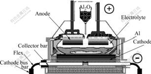
Fig.1 Schematic diagram of prebaked aluminum reduction cell

Fig.2 Sketch of basic connecting mode

Fig.3 Equivalent circuit diagram of basic connecting mode
The current flowing along each flex can be obtained as shown in Fig.4 at a given electrical potential if the resistances of three flexes are equal and the starting point of each flex is equipotential.
From Fig.4, it can be seen that with increase of the number of flexes, the current increase, if there are more flexes in a group, the trend will continue, which will increase the current difference among flexes in a group. In other words, the difference of current flowing out of collector bars will grow. Obviously, the uniform current cannot be obtained.

Fig.4 Current distribution of basic connecting mode with uniform resistance
It is expected that current distribution can be improved by adjusting the resistance arrangement of flexes in a group, so the following deduction was performed.
In Fig.2, R1, R2 and R3 represent the resistance of flexes No.1, 2 and 3 respectively. Let R�� be the resistance of the cathode bus bar between two flexes, the following resistance relation can be obtained when the same current flows out of each flex:
R2=R1+R�� (4)
![]() (5)
(5)
3.2 Generalized mode
According to the above deduction, the relation of the generalized mode (see Fig.5) can be extended by induction as follows:
![]() (6)
(6)
where Ri is the resistance of flex No. i, the numbers are increasingly assigned along the direction of current (see Fig.5).
From Eqn.(6), it can be seen clearly that the larger the number of the flex is, the larger the resistance should be assigned.
According to Eqn.(6), the resistance optimization method of the flexes in a group can be obtained including the following steps:
1) select the object to be optimized and then number the flexes as shown in Fig.5;
2) estimate the resistance of flex No.1, R1;
3) the resistance of other flexes can be calculated by using Eqn.(6).
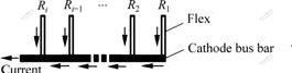
Fig.5 Schematic diagram of generalized mode extended from basic connecting mode
3.3 Extension method
According to the position where current flows out, the basic connecting mode(see Fig.2) can be extended to two other modes as follows besides the mode with the current flowing-out point on the side of the flexes(see Fig.5).
Mode 1: The mode with current flowing-out point on the side (see Fig.5). This mode is exactly the generalized mode extended from basic connecting mode (see Fig.2), the resistance of flexes can be arranged according to the method above.
Mode 2: The mode with current flowing-out point in the middle of two flexes (see Fig.6). This mode can be regarded as the combination of two parts of mode 1 on both sides, so the resistance of each side can still be arranged separately using the above calculation method, but all the flexes on both sides belong to the same group, the current flowing out of flexes on each side should be guaranteed to be equal. So, by deduction, the following equations can be used to calculate the resistance of this kind of connecting mode.
![]() (7)
(7)
![]() (8)
(8)
![]() (9)
(9)
where i��j.
First, fix the resistance of flex when i equals 1, the resistances of other flexes on this side can be calculated based on Eqn.(7), until Rmax(i) is obtained, and the Rmax(j) can be calculated by Eqn.(8) , then the other resistance of this side can be calculated by Eqn.(9).
Mode 3: The mode with current flowing-out point aligning with a flex (see Fig.7). Mode 3 is similar to mode 2, the only difference is that the current flowing-out point aligns with a flex, the flexes resistances of this mode can be calculated by the following equations:
![]() (10)
(10)
![]() (11)
(11)
![]() (12)
(12)
where i��j.
Likewise, fix the resistance of flex when i equals 1, the resistances of other flexes on this side can be calculated based on Eqn.(10), until Rmax(i) is obtained, and the Rmax(j) can be calculated by Eqn.(11), then the resistance of other flexes on this side can be calculated by Eqn.(12).

Fig.6 Schematic diagram of mode with current flowing-out point in middle of two flexes

Fig.7 Schematic diagram of mode with current flowing-out point aligning with flex
4 Example
4.1 Model development
Based on 350 kA aluminum reduction cells, a 3D finite element model for solution of electric field was developed to show the effect of the method.
In Fig.8, the model includes cathode blocks, collector bars, flexes, cathode bus bars of cell No.1; anode risers, anode beams, anode stubs, anodes, the electrolyte, and liquid-Al of cell No.2.
Cathode blocks, collector bars, anode, electrolyte and liquid-Al were meshed with hexahedron finite elements, and the bus bar system, anode beams and anode stubs were built with 2D wire bar. The temperature dependant material properties were considered (see Table 1).
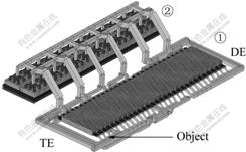
Fig.8 Finite element model of 350 kA prebaked aluminum reduction cells for solution of electric field
Table 1 Electrical conductivities of materials

4.2 Boundary conditions
Because of the complexity of cells, the boundary condition is one of the most difficult factors that affect the accuracy of simulation. The bottom surface of metal pad was assumed as the equipotential face in this model.
First, zero electric potential was applied on the bottom surface of the metal pad in cell No. 2, the excitation current of 350 kA was applied uniformly on the top surface of cathode blocks in cell No.1, then the voltage of whole model can be computed according to the material properties and resistance distribution.
After the first solution of voltage, the boundary conditions can be specified as follows:
1) zero electric potential was applied on the bottom surface of metal pad in cell No.2;
2) the voltage above was applied on the top surface of cathode blocks in cell No.1.
4.3 Solution and results
The first group of flexes (from TE to DE) of the upstream side was selected as the research object in Fig.8. And it includes five flexes simply sketched and numbered as shown in Fig.9.
A few of comparisons were made to investigate the influence of resistance of flexes, so three cases were selected for the analysis.
Case 1: The resistances of the five flexes are completely the same.
Case 2: The resistance configurations of flexes No.1, 2 and 3 are the same with small resistance, while the configurations of flexes No.4 and 5 are the same with large resistance.
Case 3: The resistance of each flex is different. The resistances of the flexes are obtained and assigned according to model 1.
During the analysis, only the resistance of the object in the model was modified, and the other parts of the model including the boundary conditions were kept at constant. The result of each case is shown in Fig.10. From Fig.10, it can be seen that in case 1 with increasing number of flexes, the current increases, the difference between the maximum and minimum current is 180.6 A. In case 2, because the resistances of flexes No.4 and 5 are modified, the current reduces from flex No.4 firstly and then increases in turn and the difference between the maximal and minimal is 78.2 A. In case 3, the current distribution of each flex is uniform, but due to the difference of electric potential at the end of each collector bar, the current still fluctuates. The difference between the maximal and minimal current is 25.4 A.

Fig.9 Schematic diagram of the first group flexes

Fig.10 Comparison of results of different cases
4.4 Discussion and suggestion
The calculation method of resistance of flexes was deduced in an ideal situation. It is beneficial to calculating and designing the resistance of each flex based on this method. In order to reduce its complexity, the resistance of flexes can be adjusted piecewise using the method, as case 2 shown in Fig.10. This configuration can also improve the current distribution of collect bars as shown in Fig.2. This method can balance the current of each collector bar without increasing the cost too much.
By comparing the modes in Figs.5-7, it can be seen that with the same number of flexes, the range of resistance adjustment of mode 1 is smaller than those of modes 2 and 3. Therefore, if there are many flexes in a group, it may be difficult to adjust the resistance by choosing mode 1, but mode 2 or 3 may be preferred.
Specially, to obtain uniform current distribution, when the number of flexes in a group is odd mode 3 is the best, and when the number of flexes in a group is even mode 2 is the best.
It is known that the resistance is adjusted by changing the length and cross section area of the conductor, but they are restricted by a lot of factors in practice. The investment, expense and the process of exceptional errors must be considered especially, so the appropriate current mode and resistance configuration should be decided suitably according to actual needs.
5 Conclusions
1) Three flex connecting modes are generalized. The ideal resistance relationship formulas among the flexes, which can make current evenly distributed in every local flex, are obtained for each mode.
2) The effect of the resistance optimization method is validated by a 350 kA aluminum reduction cell based electric field model. Current variation decreases in local flexes after the method is used. The method is of importance to design the improved bus bar configurations.
References
[1] ZHOU Nai-jun, XIA Xiao-xia, WANG Fu-qiang. Numerical simulation on electrolyte flow field in 156 kA drained aluminum reduction cells[J]. Journal of Central South University of Technology, 2007, 14(1): 42-46.
[2] LIU Wei, LI Jie, LAI Yan-qing, LIU Ye-xiang. 2D finite element analysis of thermal balance for drained aluminum reduction cells[J]. Journal of Central South University of Technology, 2007, 14(6): 783-787.
[3] TVEDT T, NEBELL H G. Newbus, a simulation program for calculation of the current distribution in the bus bar system of alumina reduction cells[C]// BOXALL L G. Light Metals 1988. Phoenix, Arizona: TMS, 1988: 567-573.
[4] BUIZA J I. Electromagnetic optimization of the V-350 cell[C]// CAMPBELL P G. Light Metals 1989. Las Vegas, Nevada: TMS, 1989: 211-214.
[5] YAO Shi-huan, HE Zhi-hui. Selection of bus bar optimum section in high amperage reduction cells[C]// Bickert C M. Light Metals 1990. Anaheim, California: TMS, 1990: 453-458.
[6] SEVERO D S, SCHNEIDER A F, PINTO E C V, GUSBERTI V, POTOCNIK V. Modeling magnetohydrodynamics of aluminum electrolysis cells with ANSYS and CFX[C]// KVANDE H. Light Metals 2005. San Francisco, California: TMS, 2005: 475-480.
[7] DUPUIS M, BOJAREVICS V, FREIBERGS J. Demonstration of thermo-electric and MHD mathematical models of a 500 kA Al electrolysis cell: Part 2[C]// ALTON T T. Light Metals 2004. Charlotte, North Carolina: TMS, 2004: 453-459.
[8] DUPUIS M, BOJAREVICS V. Weakly coupled thermo-electric and MHD mathematical models of an aluminium electrolysis cell[C]// KVANDE H. Light Metals 2005. San Francisco, California: TMS, 2005: 449-454.
[9] KACPRZAK D, GUSTAFSSON M J, TAYLOR M P. A finite element analysis of busbars and magnetic field of an aluminum reduction cell[J]. IEEE Transactions on Magnetics, 2006, 42(10): 3192-3194.
[10] DUPUIS M. Using ANSYS to model aluminum reduction cell since 1984 and beyond[C]// PETERSON R D. Light Metals 2000. Nashville, Tennessee: TMS, 2000: 307-313.
[11] ZHOU Nai-jun, MEI Chi, JIANG Chang-wei, ZHOU Ping, LI Jie. Coupled computation method of physics fields in aluminum reduction cells[J]. Transactions of Nonferrous Metals Society of China, 2003, 13 (4): 431-437.
[12] LI Jie, CHENG Ying-jun, LAI Yan-qing, ZHOU Nai-jun. Numerical simulation of current and temperature fields of aluminum reduction cells based on ANSYS[J]. Chinese Journal of Computation Physics. 2003, 20(4): 351-355. (in Chinese)
[13] YANG Yi, LI Lang-ru. Magnetic field analysis of large aluminum reduction cell by using finite element method[J]. Nonferrous Metals, 2002, 8(3): 66-69. (in Chinese)
[14] JIANG Chang-wei, MEI Chi, ZHOU Nai-jun, XU Shun-sheng. Computation of 3-D magnetic field in prebaked cells using scalar voltage potential method and two scalar magnetic potentials method[J]. The Chinese Journal of Nonferrous Metals, 2003, 13(4): 1021-1025. (in Chinese)
[15] LIU Hai-shi, LI Jie, LI Cui-mei, ZHANG Qin-song, LIU Wei. Influence of different kinds of cathode carbon blocks on cathode thermal-field distribution in preheating process[J]. Journal of Central South University: Science and Technology, 2006, 37(1): 36-40. (in Chinese)
[16] WU Jian-kang, HUANG Min, HUANG Jun, YAO Shi-huan. Computation of flow field of electrolyte-aluminium liquid and surface distortion of aluminum liquid in reduction cell[J]. The Chinese Journal of Nonferrous Metals, 2003, 13(1): 241-244. (in Chinese)
[17] DUPUIS M, BOJAREVICS V. Busbar sizing modeling tools: Comparing an ANSYS based 3D model with the versatile 1D model part of MHD-Valdis[C]// GALLOWAY T J. Light Metals 2006. San Antonio, Texas: TMS, 2006: 341-346.
[18] KACPRZAK D, GUSTAFSSON M J, LI L, TAYLOR M. Numerical analysis of the collector bar current distribution of a reduction cell[C]// GALLOWAY T J. Light Metals 2006. San Antonio, Texas: TMS, 2006: 367-369.
Foundation item: Project(60634020) supported by the National Natural Science Foundation of China
Received date: 2007-08-02; Accepted date: 2007-09-16
Corresponding author: LI Jie, Professor; Tel: +86-731-8830474; E-mail: 13808488404@hnmcc.com
