
���±�ţ�1004-0609(2015)-11-3182-08
������С�ݶ�֧�ŵ�2.5D���ص�λ�����۽�����
��־��1���� ��2��������2
(1. ���ϴ�ѧ �����ѧ����Ϣ����ѧԺ����ɳ 410083��
2. ����������ѧ ����Դ�뻷���������ص�ʵ���ң��ϲ� 330013)
ժ Ҫ��
������С�ݶ�֧���ȶ����ӽ���2.5D���ص�λ�۽����ݡ�ͨ���Ա߽���ƴ�������ϻ���ͼ�����۵ľ�������������Ԫ����������ʵ��һ�ֿ��ٵ�����ϡ�����ֱ�ӷֽⷽ������������ݼ���Ч�ʡ�Ϊ��ͻ���Զ����쳣��߽��ʶ��������������С�ݶ�֧���ȶ�����(MGS)�������ؼ�Ȩ�����ݶ�(RRCG)�������з���Ŀ�꺯����⡣���������MGS�������õľ۽�������RRCG���ݵ��������ȶ��������ٶȿ졣�ԡ�L-curve��ѡ���������ӵ��㷨���иĽ��������˴�ͳ����������ʼ���ʱ��Ҫ����ɢ�������������ͬʱ���㷨���ڳ��ֶ���յ�ġ�L-curve��Ҳ����ȷѡ���������ӡ�
�ؼ��ʣ�
���ص�λ�����ؼ�Ȩ�����ݶȷ��� L-curve����С�ݶ�֧���ȶ�������LDLT�ֽ��㷨��
��ͼ����ţ�P631���� ���ױ�־�룺A
2.5D focusing inversion for borehole-surface electrical data based on minimum gradient support function
ZHANG Zhi-yong1, ZHOU Feng2, LI Ze-lin2
(1. School of Geosciences and Info-Physics, Central South University, Changsha 410083, China;
2. Key Laboratory of Nuclear Resources and Environment, Ministry of Education,
East China Institute of Technology, Nanchang 330013, China)
Abstract: The 2.5D focusing inversion for borehole-to-ground electric potential was implemented using minimum gradient support function. The boundary approximation, matrix rearrangement and fill-in element analysis algorithm based on graph theory were adopted to complete the fast algorithm of direct decomposition method for sparse matrix, the computational efficiency was improved. In order to improve the inversion ability to discriminate boundary of abnormal bodies, the minimum gradient support stability factor (MGS) was adopted. On the other hand, re-weighted regularized conjugate gradient (RRCG) inversion method was applied to solve inverse function. The results show that the stability factor is good at invert sharp boundary of underground bodies, RRCG method is stable and fast. For the rapid selection of the most suitable regularization factor, the revised ��L-curve�� algorithm was studied. New method based on the simply principle of distance from point to line, the error caused by the derivation of discrete data was avoided when the regularization factor was calculated using the maximum curvature method, moreover, for multiple inflection point of the ��L-curve��, it also can select the best regularization factor.
Key words: borehole-surface electrical method; re-weighted regularized conjugate gradient; L-curve; minimum gradient support function; LDLT factorization
ֱ�������ʷ��ǿ����Դ���顢ˮ��Դ����ij��÷���֮һ���������ر����ڻ����빤�̵��������еõ��㷺Ӧ�á�ֱ�������ʷ������õر��۲⣬ͨ���ӵ��������������ͼ�Ե���Ŀ��������ƶϽ��͡���ijЩ����£����ڲ�����Ŀ��������ʲ�������ƣ�����Ӱ��̽�������ֱ��ʣ����ص編���ھ��е缫�����룬�������˴�ͳ�����IJ��㣬���Ǿ��ص�λ�������ڲ����Ӳ��������ͼ��ʾ����ˣ����Ͻ����������ݼ�������ǰ���ص�λ�����뷴�ݳ�Ϊ���о����ȵ�[1-6]��SCRIBA[7]��SPITZER[8]���ñ߽�Ԫ��ʵ������ά���ص�λ����ģ�⣻PRIDMORE ��[9]��������Ԫ��ʵ����ά���ص�λ����ģ�⣻�쿭����[10]����־�յ�[11]���������ʵ���˴�ֱ��Դ���ص�λ����ά����ģ�⣻��ǰΰ��[12]�����˾��ص�λ2.5����Ԫ��ֵģ���쳣�����������µ�[13]�����˿ӵ��ڵľ۽���ǰ̽������ʷ�����Ԫ��ֵģ���о���LI��[14]�����˵���;��й۲����ݵ���ά�����о����¸��ʵ�[15]Ӧ�÷�����������С���˵����㷨ʵ���˾��ص編����ά�������о�����������[16]�����˹����ݶȷ������С����Ŀ�꺯��ʵ���˾�����ά�������ݵĿ��ٷ��ݣ���־�յ�[17]ʵ����Born���ƿ�����ά���ص編���ݵķ��ݣ���Ȼ��[18]ʵ���˾�����ά�����ʷ��ݡ�
������֪������������������ڲ��ȶ��������ԣ��������ǵõ��ȶ������Ҫ����֮һ��������ͨ���ڷ���Ŀ�꺯���������ȶ����ӣ���ģ�ͽ�ռ����Լ�������ٷ�����IJ��ʶ��ԡ����������г��õ��ȶ�������ʽ�У���Сģ��Լ�������ƽ��ģ��Լ����ģ���ܱ仯��Լ������С֧��Լ������С�ݶ�֧��Լ���ȡ�CONSTABLE��[19]��SMITH��[20]��ZHDANOV��[21-22]�ɹ��ؽ����ƽ��ģ��Լ��Ӧ�õ������������ݽ��ͣ����У���CONSTABLE��[19]��DEGROOT-HEDLIN��[23]�����OCCAM�����㷨Ӧ����Ϊ�㷺��RUDIN��[24]�ڶ�ͼ��߽��ʶ���о��������ģ���ܱ仯��Լ�����÷�ͨ��ģ�Ͳ����ݶ��ڶ�������L1������С����Լ����ʶ��߽磻GAO��[25]��ģ���ܱ仯��Լ��Ӧ�õ�����ӫ������У�BURSTEDDE��[26]��һάȫ����������Ҳ������ģ���ܱ仯��Լ����������[27]���ģ���ܱ仯���;������������ŵ㣬ʵ���˵����ʳ���Ļ���������㷨��Ϊ�˼�������ľֲ��������壬LAST��[28]�����С���֧��Լ����Ӧ�����������Ϸ��ݽ��ͣ�֮��GUILLEN��[29]��BARBOSA��[30]����һ�������иĽ���ʹԼ���������з����ԣ�CANDANSAYAR[31]��MEHANEE��[32]��PORTNIAGUINE��[33]��������MT���ݷ��ݣ�GRIBENKO��[34]��������CSEM��ά���ݣ�VIGNOOLI��[35]��������С֧���ȶ������Ц�ȡֵ�Է��ݽ����Ӱ�졣��С�ݶ�֧��Լ����һ������ͻ������߽�ʵ�־۽����ݵ�Լ����ʽ��������PORTNIAGUINE��[36]�����Ӧ�õ��������������У�֮��ZHDANOV��[37]ʵ���������ľ۽����ݣ�SALAH[38]ͬ�����˷���Ӧ�õ�������ģ�ͷ��ݣ���С����[39]�����˶�ά��ص�����ݵľ۽������㷨�о���
�����Ǿ���λ�����ݴ����ĺ��ģ�ֱ��Ӱ��������Ͻ��͡�Ϊ����߶���߽�������ʶ���������������߲�����С�ݶ�֧�ŵ��ȶ�����ʵ���˾۽����ݡ�Ϊ������ٶȣ������˻�����С����Ԫ˼���ϡ�����LDLT�ֽ��㷨��Ϊ�˿��پ�ȷѡ���������ӣ��о���L-curve���Ľ��㷨���������������ʹ����ж���ɢ������������������ؼ�Ȩ�����ݶȷ�(RRCG)�������Ŀ�꺯��[36]����������ȶ����������ٶȣ��Ҹ÷���ֻ���ڳ�ʼ����ʱѡ��һ���������ӣ��ں���ĵ������Զ������������������������÷������нϺõĶ���߽�ʶ�����������õ�Ӧ��ǰ����
1 ���ص�λ��������
ֱ����������ά����Ե���������(z����)���и���Ҷ�任���õ�2.5D���ص�λ�ı�ֵ����[40]�������ʽΪ
 (1)
(1)
ʽ�У�����Ϊ��ά�о�����s������Ϊ��ά����ı߽�(��sΪ���ĵر��߽磬����Ϊ���ĵ��±߽�)����Ϊ�絼�ʣ�rΪ���Դ���߽�ľ��룻nΪ�߽��ⷨ����kΪ���ϱ任��������Ϊ�߽��ⷨ�����빩��㵽�߽�ʸ���нǣ�K0��K1�ֱ�Ϊ��ס�һ�ڶ������������(xs��ys)��ʾxyƽ���ϵĹ�������ꣻ��(x)��ʾ��x��Ϊ���ĵ�һά�����˺�����IΪ����������
Ϊ�˸��õ�ģ����µ��������̬��������ݼ���ľ��ȣ����������ǵ�Ԫ˫���β�ֵ����Ԫ����⡣ʽ(1)�ı�ֵ���������ʽ(2)�ı������ȼۡ�

 (2)
(2)
ͨ����ʽ(2)������ɢ���õ����Է����飺
KU=P (3)
���ʽ(3)������ý���ϸ������λ��ͨ������Ҷ���任�õ���λu���о��������ð˵��˲�ϵ�����и���Ҷ�任�����任�����任ϵ��(km)�뷴�任ϵ��(gm)���1����[41]��
��1 ���ϱ任ϵ��km��gm
Table 1 km and gm parameters of Fouriers inverse transform

����ʽ(2)��֪����������ֳ�Ŀ�����ͱ߽�����Ŀ����Ϊ�쳣����ڵ��������������õȾ��ʷ֣��߽�������������ָ����������ʽ��ģ������߽硣���ڲ���ָ�����ߣ�����㵽�߽��ʸ��r��Լ�����Ŀ�����㹻����ˣ��ɲ���Ŀ�������ĵ��߽��ʸ�����ƣ������նȾ���ֻ�벨���йأ����빩����ء�������һ�ص㣬Ϊ��������Ч�ʣ���ϻ���ͼ�����۵ľ�������������Ԫ�����㷨�������ϡ������LDLT�ֽ��㷨������ȷ�����ʷ���ʽ��ֻ��һ�λ�����������Ԫ�ķ��ŷ���[42] ������ͬһ����ֻ��һ��LDLT�ֽ��㷨�������������ݵļ����ٶ�Ϊ�����о��춨�˻������������������ͼ1��ʾ��
2 ���ص�λ�۽�����
�����Ǿ��ص�λ���Ͻ��͵���Ҫ���ڡ�Ϊʵ�ֶ���߽�����巴�ݣ��о��˻�����С�ݶ�֧���ȶ����ӵ������ݼ������������ӵ�ѡ����Ŀ�꺯�������Ż�����������ݵ������ؼ����ڣ����������ڡ�L-curve�������������һ�ָĽ��ġ�L-curve��������ʵ�����������ӿ���ѡ����RRCG������ⷴ��Ŀ�꺯��������˷��ݹ��̵��ȶ��������Ч�ʡ�
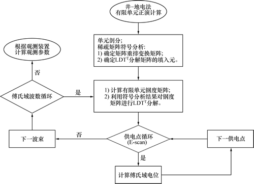
ͼ1 ���ص�λ����Ԫ���ݼ�������
Fig. 1 Flow chart of borehole-surface electrical numerical simulation using FEM
2.1 ������С�ݶ�֧�ŵ�������
Tikhonov����
 (4)
(4)
ʽ�У�P(����m)ΪĿ�꺯������Ϊ��������(Regularization parameter)����d(m)Ϊ����Ŀ�꺯������m(m)Ϊģ��Լ��Ŀ�꺯����Ҳ���ȶ�����(stabilizer) [21]��mΪģ�Ͳ�����
ͨ������ʵ��������Ԥ�����ݵľ�������ʾ��d(m)����

 (5)
(5)
ʽ�У� Ϊ����Ȩ�ؾ���A(m)���ݺ�����dΪ�۲����ݡ�
ZHDANOV��[21]������С������ʽ������һ���ȶ����ӵ�ͳһ��ʾ��ʽ����Сģ���ȶ�����������õ��ȶ�������ʽ���������˵�ǰģ�ͺ�����ģ��֮���L2������ģ��Լ��Ŀ�꺯���ı���ʽΪ

 (6)
(6)
ʽ�У�maprΪ����ģ�ͣ� Ϊģ��Ȩ�ؾ��������ʽ(6)Ϊ����ʽ��ͨ���������
 ����Եõ���ͬ�ȶ����ӵ�ͳһ��ʾ��ʽ[33]��
Ϊʵ�ֶ����쳣��ı߽練�ݣ�PORTNIAGUINE��[36]�������С�ݶ��ȶ����ӣ�
 (7)
(7)
ʽ�У���Ϊ�۽����ӡ�������֪��ʽ(7)��Ϊ�ȶ����ӽ�ͻ��ģ���ݶȵı仯���Ӷ�ʵ�־۽����ݡ�
Ϊ������ʽ(7)ͳһ��ʾ�ȶ����ӣ�����ʽ(7)����ģ��Ȩ�غ�����

 (8)
(8)
ʽ�У�m(r)Ϊģ�Ͳ����ֲ������� Ϊģ�Ͳ����ݶȣ�eΪ��������ֵ�����йص�һ����С������
Ȼ��ʽ(5)��(6)��(8)���뵽ʽ(4)�У���

 (9)
(9)
���ɵõ�������С�ݶ�֧���ȶ����ӵ�������Ŀ�꺯����
2.2 �ؼ�Ȩ�����ݶȷ�(RRCG)
�����ؼ�Ȩ�����ݶȷ����ʽ(9)��ʾ���Ż����⣬�÷�����ÿһ�ε�������������ǰһ�μ��� �õ���ģ���������¼���Ȩ�ؾ��� ����
����  ��
�� Ϊ��n�ε�����ģ���������ؼ�Ȩ�����ݶȷ�ģ����Ϊ
 (10)
(10)
ʽ�У� Ϊ���������ĵ���������
 Ϊ�����ݶ���������������
 (11)
(11)
ʽ�У� Ϊ��n�������������½������������ɱ�ʾΪ
 (12)
(12)
ʽ�У� Ϊ��n�ε�����ƫ���������ݹ����ݶȷ������������������
 (13)
(13)
Ϊȷ��ʽ(10)ÿһ������Ŀ�꺯������½������������ĵ�������Ϊ
 (14)
(14)
���⣬��n=0ʱ����
 (15)
(15)
Ϊȷ��Ŀ�꺯���½������������ȶ����ӽ���������������Ӧ������

 (16)
(16)
����
 (17)
(17)
���ݦÿ�ʵ���������ӵ��Զ���������
 (18)
(18)
2.3 ������L-curve������
�������Ӧ�������Ŀ�꺯����ģ��Լ�������ļ�Ȩϵ�����Ƿ��ݵĹؼ�����֮һ��HANSEN[43]����á�L-curve��(��ͼ2(a))��ȷ���������ӣ��÷���ͨ����ȡ˫���������� ��
�� �����������
 ��ȷ���������Ӧ���˫�������������������ʿɱ�ʾΪ
 (19)
(19)
ʽ�У� ��
�� ��
�� Ϊ
Ϊ ��
�� ��һ�������ڷ��ݹ����У���������ɢ�ģ��䵼��ֻ��ͨ����ֵ�������㣬���Ȳ��ߣ�����Ӱ����
 ֵ�����⣬��ʵ�������з���˫���������������߲������dzʡ�L���Σ��ܶ�����±���Ϊ�����յ�(��ͼ2(b))��
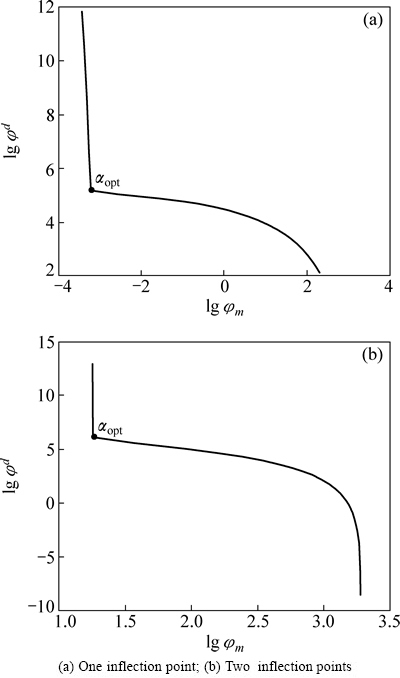
ͼ2 L-Curve����ͼ
Fig. 2 L-curve feature map
����������������ˡ�L-curve���ĸĽ��㷨�������ԭ���ǻ��ڵ���ֱ�ߵĹ�ϵ�����õ㵽ֱ�ߵľ�����м��㣬�㷨���岽�裺
1) ������ʼ���������� �����ʽ(9)�õ�
 ���������Ӧ��
 ��
��
2) �� ����
���� ��
�� �ֱ���3��������ֵ���ֱ�ֵ������Ϊ
 ��
�� ��
��
3) ȡ��L-curve���ϵ������˵㣬����ֱ�߱���ʽ ��
��
4) ȡ��L-curve���ϵ������ ���������ֱ�߱���ʽM�У�����
 ��
��
5) ����������ֱ��M�ľ���{dk}��ɸѡ���������ĵ�dh��
6) ������ �����ʷ֣���Ϊ��ʼֵ���¼��㲽��1)~����5)��ֱ����������������
�Ľ��ġ�L���ߡ��㷨�����������ĵ�����Ϣ�������Զ������������ʵ㣬������������ӵ���ȡ���ȡ�
3 ������������
3.1 ģ������
���Ȱ�ռ��д���һ������L���͵ĵ����쳣��(��ͼ3)�������쳣��ĵ�����Ϊ50 ����m������������Ϊ100 ����m����ˮƽ����10 m��20 m���辮�е缫(��32����ÿ�ھ�16��)���ر�����30���缫������������ģ�����ݽ������2%��������õ����ֱ������С�ݶ�֧�š���ƽ��ģ�ͼ���Сģ���ȶ����ӽ��з��ݣ����ݶ�����ͼ4��ʾ�������ȶ����Ӿ��ܷ�ӳ�����쳣��Ĵ��ڣ���С�ݶ��ȶ����ӵõ��ķ��ݽ����������ȶ����ӣ��߽�����ԣ����ұ��������ʽӽ�100 ����m�����������ȶ����ӣ����ݶ�����ڶദ���쳣���쳣��߽�Ķ���̶��ܵ���λ�õ�Ӱ�죬�뾮Խ���߽�Խ���ԡ�

ͼ3 ģ��ʾ��ͼ
Fig. 3 Schematic diagram of model

ͼ4 ���ݵ����ʶ���
Fig. 4 Inversion resistivity sections
3.2 ij����Ĺ���������淴��
���ﱣ����λ��ij����Ĺ�������б������ھ�Ϊȷ��Ĺ�ҡ�����ӡ�Ĺ����λ�ü��Ƿ���ڹŴ������������������ֱ���編��̽��������������̽������У�����һ�����������չ�˾��ص編�������ر�����2.5 m���࣬������60���缫�������в���1.0 m���࣬�����þ��е缫8��(�缫λ�ü�ͼ5�����в����ڷ�������ĵر��缫δ����)��������С�ݶ��ȶ����ӵ�������Ŀ�꺯����Ӧ��RRCG���������˷��ݣ����ݵ����ʶ�����ͼ5��ʾ��
�ӵر������ƶϣ������߳���ߵĵط�(ˮƽ����20~32 m��55~75 m)Ϊ��Ĺ������Ĺ�ķ����������·�Ӧ������Ĺ�ҡ����������ѵ����Ϸ������ڴ�����������У��Ҳ�����Ͼã����ݵ��ذ��շ�ӳ���ܷ�����20����80��������������ڿ��ڻ�û�дﵽĹ�ң�������Ҳ�����ò��þ��е缫�ĵ������ɷ��ݵ����ʶ���(��ͼ5)��֪���ö�������ʱ仯��ΧΪ40~400 ����m�����иߵ�������(��280 ����m)��Ҫ�ֲ��ڸ߳̽ϸߺ͵��α仯���λ�ã��Ʋ���Ҫ��������Щ������������ˮ�Ƚϸ������ɣ�-10 m����Ϊ�͵�������(��100 ����m)�����ˮ�ĵ��������Ʋ⣬�����DZˮ���йأ��Ҳ��������160~220 ����m�İ�Χ���ڴ���220~280 ����m�ķ���쳣���Ʋ��м����쳣ΪĹ�ң�Ĺ����Χ�ĸ����Ʋ��뺻����ʩ���йأ�����������100~160 ����m�İ�Χ���ڴ���40~100 ����m�ķ���쳣���Ʋ��м�������쳣ΪĹ�ҡ���������Ĺ�ҷֱ����Ϊ�������и��裬���ֳ����鷢�֣��������ڲ���ˮ�����Ҳ�����ڲ���Ϊ���

ͼ5 �����淴�ݵ����ʶ���
Fig. 5 Inversion resistivity section of mainly survey line
4 ����
1) ���Ƶı߽紦���Լ����ڷ��ŷ�����LDLT�ֽ��㷨��������������ݼ���Ч�ʣ�Ϊ���ٷ��ݵ춨������
2) ���øĽ��ġ�L-curve����ȡ�������ӣ����㷽�㣬�������ɢ����������˷��ݵ��ȶ��ԡ�
3) �ؼ�Ȩ�����ݶȷ���ͨ����ÿ�ε��������У������Ȩ�ؾ�������������ǰһ���ȶ������뱾���ȶ����ӵı�ֵ��Ϊ�������ӵ�˥��ϵ�������ֵ�������������Ӧ��ȡ�������ӵķ�������˷���Ч�ʼ�������ȶ��ԡ�
4) ��С�ݶ�֧���ȶ��������������2.5D���ط��ݶ����쳣��߽��ʶ��������
REFERENCES
[1] SMITH N C, VOZOOFF K. Two-dimensional DC resistivity inversion for dipole-dipole data[J]. IEEE Transactions Geoscience Remote Sensing, 1984, 22(1): 21-28.
[2] ZHOU B, GREENHALGH S A. A synthetic study on cross-hole resistivity imaging with different electrode arrays[J]. Exploration Geophysics, 1997, 28(2): 1-5.
[3] ZHANG J, MACKIE R L, MADDEN T R. 3-D resistivity forward modeling and inversion using conjugate gradients[J]. Geophysics, 1995, 60(5): 1313-1325.
[4] OLDENBURG D W, MCGILLICRAY P R, ELLIS R G. Generalized subspace methods for large-scale inverse problem[J]. Geophysical Journal International, 1993, 114(1): 12-20.
[5] LI Y G, OLDENBURG D W. Approximate inverse mapping in DC resistivity problems[J]. Geophysical Journal International, 1992, 109(2): 343-362.
[6] MAURIELLO P, PATELLA D. Resistivity anomaly imaging by probability tomography[J]. Geophysical Prospecting, 1999, 47(3): 411-429.
[7] SCRIBA H. Computation of the electrical potential in the three-dimensional structures[J]. Geophysical Prospecting, 1981, 29(5): 790-802.
[8] SPITZER K. 3-D finite-difference algorithm for DC resistivity modeling using conjugate methods[J]. Geophysical Journal International, 1995, 123(3): 903-914.
[9] PRIDMORE D F, HOHMANN G W, WAED S H, SILL W R. An investigation of finite-element modeling for electrical and electrical and electromagnetic data in three dimensions[J]. Geophysics, 1981, 46(7): 1009-1015.
[10] �쿭��, ��ͩ��. ��ֱ������Դ��ά�ص糡����������о�[J].���ִ�ѧѧ��(�����ѧ��), 2006, 36(1): 137-141.
XU Kai-jun, LI Tong-lin. The forward modeling of three-dimensional geo-electrical field of vertical finite line source by finite difference method[J]. Journal of Jilin University (Earth Science Edition), 2006, 36(1): 137-141.
[11] ��־��, ��չ��, κ�IJ�. ����ֱ���編��ά��ֵģ�������������о�[J]. ��̽��̽���㼼��, 2006, 28(4): 322-326.
WANG Zhi-gang, HE Zhan-Xiang, WEI Wen-bo. Study on some problems upon 3D modeling of DC borehole-ground method[J]. Computing techniques for geophysical and Geochemical Exploration, 2006, 28(4): 322-326.
[12] ��ǰΰ, ���dz�, ���黪. ���ص�λ2.5ά����Ԫ��ֵģ���쳣����[J]. ��̽��̽���㼼��, 2013, 35(4): 457-462.
DAI Qian-wei, HOU Zhi-chao, WANG Hong-hua. Anomalous analysis of the 2.5D finite element numerical simulation of borehole-ground electrical method[J]. Computing Techniques for Geophysical and Geochemical Exploration, 2013, 35(4): 457-462.
[13] ������, ��С��, ������, ������, ͯТ��, �� . �ӵ�ֱ���۽���ǰ̽������ʷ�����Ԫ��ֵģ��[J]. �й���ɫ����ѧ��, 2012, 22(3): 970-975.
LIU Jian-xi, DENG Xiao-kang, GUO Rong-wen, LIU Hai-fei, TONG Xiao-zhong, LIU Zhuo. Numerical simulation of advanced detection with DC focus resistivity in tunnel by finite element method[J]. The Chinese Journal of Nonferrous Metals, 2012, 22(3): 970-975.
[14] LI Y G, OLDENBURG D W. 3-D inversion of induced polarization data[J]. Geophysics, 2000, 65(6): 1931-945.
[15] �¸���, ���廪. ���ص編����ά�������о�[J]. ������ѧѧ��(��Ȼ��ѧ��), 2009, 45(3): 264-272.
KE Gan-pan, HUANG Qing-Hua. 3D Forward and inversion problems of borehole to surface electrical method[J]. Acta Scientiarum Naturalium Universitatis Pekinensis, 2009, 45(3): 264-272.
[16] ������, ���Ң, �ƿ���. ֱ���羮����άֱ�ӳ���[J]. ��̽��̽���㼼��, 2003, 25(1): 60-64.
 Yu-zeng, RUAN Bai-yao, HUANG Jun-ge. The 3-D immediate cross hole tomography with direct current[J]. Computing Techniques for Geophysical and Geochemical Exploration, 2003, 25(1): 60-64.
[17] ��־��, ��չ��, κ�IJ�. Born���ƿ�����ά���ݾ��ص編����[J]. ��������ѧ��չ, 2007, 22(2): 508-513.
WANG Zhi-gang, HE Zhan-xiang, WEI Wen-bo. Fast 3D inversion of borehole ground electrical method data based on born approximation[J]. Progress in Geophysics, 2007, 22(2): 508-513.
[18] �� Ȼ, ��ͩ��, �쿭��. ������ά�����ʷ����о�[J]. ��������ѧ��չ, 2007, 22(1): 247-249.
AN Ran, LI Tong-lin, XU Kai-jun. Well-surface 3-D resistivity inversion[J]. Progress in Geophysics, 2007, 22(1): 247-249.
[19] CONSTABLE S C, PARKER R L, CONSTABLE C G. Occam��s inversion: A practical algorithm for generating smooth models from EM sounding data[J]. Geophysics, 1987, 52(3): 289-300.
[20] SMITH J T, BOOKER J R. Rapid inversion of two- and three-dimensional magnetotelluric data[J]. Journal of Geophysical Research: Solid Earth, 1991, 96(3): 3905-3922.
[21] ZHDANOV M S. Geophysical inverse theory and regularization[M]. New York: Elsevier Science, 2002: 149-165.
[22] ZHDANOV M S, FANG S. 3-D quasi-liner electromagnetic inversion[J]. Radio Science, 1996, 4(3): 741-745.
[23] DEGROOT-HEDLIN C, CONSTABLE S. Occam��s inversion to generate smooth, two dimensional models from magnetotelluric data[J]. Geophysics, 1990, 55(12): 1613-1624.
[24] RUDIN L I, OSHER S, FATEMI E. Nonlinear total variation based noise removal algorithms[J]. Physical D: Nonlinear Phenomena, 1992, 60(14): 259-268.
[25] GAO H, ZHAO H K. Multilevel bioluminescence tomography based on radioactive transfer equation Part 2: Total variation and l1 data fidelity[J]. Optics Express��2010, 18(3): 2894-2912.
[26] BURSTEDDE C,GHATTAS O. Algorithmic strategies for full wave-form inversion: 1D experiments[J]. Geophysics, 2009, 74(6): 37-46.
[27] �� ��, �����, �� ��. �����ʳ���Ļ���������㷨[J]. ��������ѧ��, 2012, 55(3): 970-980.
HAN Bo, DOU Yi-xin, DING Liang. Electrical resistivity tomography by using a hybrid regularization[J]. Chinese Journal of Geophysics, 2012, 55(3): 970-980.
[28] LAST B J, KUBIK K. Compact gravity inversion[J]. Geophysics, 1983, 48(6): 713-721.
[29] GUILLEN A, MENICHETTI V. Gravity and magnetic inversion with minimization of a specific functional[J]. Geophysics, 1984, 49(8): 1354-1360.
[30] BARBOSA V C F, SILVA J B C. Generalized compact gravity inversion[J]. Geophysics, 1994, 59(1): 57-68.
[31] CANDANSAYAR M E. Two-dimensional inversion of magnetotelluric data with CG and SVD: A comparison study of different stabilizers[J]. SEG Technical Program Expanded Abstracts, 2002, 21(1): 669-672.
[32] MEHANEE S, ZHDANOV M S. Two-dimensional magnetoelluric inversion of blocky geo-electrical structures[J]. Journal of Geophysical Research, 2002, 107(B4): 2065-2075.
[33] PORTNIAGUINE O, ZHDANOV M S. 3-D magnetic inversion with data compression and image focusing[J]. Geophysics, 2002, 67(5): 1532-1541.
[34] GRIBENKO A, ZHDANOV M. Rigorous 3-D inversion of marine CSEM data based on the integral equation method[J]. Geophysics, 2006, 25(1): 815-819.
[35] VIGNOLI G, DEIANA R, CASSIANI G. Focused inversion of vertical radar profile (VRP) travel time data[J]. Geophysics, 2012, 77(1): 9-18.
[36] PORTNIAGUINE O, ZHDANOV M S. Focusing geophysical inversion images[J]. Geophysics, 1999, 64(3): 874-887.
[37] ZHDANOV M S, ELLIS R, MUKERJEE S. Three-dimensional regularized focusing inversion of gravity gradient tensor data[J]. Geophysics, 2004, 69(4): 925-937.
[38] SALAH A M. Multidimensional finite difference electromagnetic modeling and inversion based on the balance method[D]. Utah: The University of Utah, 2003.
[39] ��С��, ������, �� ��, �� ��. ��ά��ص�����ݵľ۽������㷨̽��[J]. ʯ�͵���������̽, 2007, 42(3): 338-342.
LIU Xiao-jun, WANG Jia-lin, CHEN Bing, YU Peng. The focusing inversion of 2-D magnetotelluric[J]. Oil Geophysical Prospecting, 2007, 42(3): 338-342.
[40] ������. ���������е�����Ԫ��[M]. ����: ��ѧ������, 1994: 159-178.
XU Shi-zhe. The Finite element method in Geophysics[M]. Beijing: Science Press, 1994:159-178.
[41] ERHAN E, ISMAIL D, MEHMET E C. Incorporating topography into 2D resistivity modeling using finite-element and finite-difference approaches[J]. Geophysics, 2008, 73(3): 135-142.
[42] LIU J. The role of elimination trees in sparse factorization[J]. SIAM Journal on Matrix Analysis and Applications, 1990, 11(1): 134-172.
[43] HANSEN P C. Analysis of discrete ill-posed problems by means of the L-curve[J]. Siam Review, 1992, 34(4): 561-580.
(�༭ �� ��)
������Ŀ��������Ȼ��ѧ��������������Ŀ(41304055��41304056��41104074)
�ո����ڣ�2015-03-17�������ڣ�2015-08-14
ͨ�����ߣ���־�£������ڣ��绰��18007910091��E-mail��zhyzhang78@hotmail.com
ժ Ҫ��������С�ݶ�֧���ȶ����ӽ���2.5D���ص�λ�۽����ݡ�ͨ���Ա߽���ƴ�������ϻ���ͼ�����۵ľ�������������Ԫ����������ʵ��һ�ֿ��ٵ�����ϡ�����ֱ�ӷֽⷽ������������ݼ���Ч�ʡ�Ϊ��ͻ���Զ����쳣��߽��ʶ��������������С�ݶ�֧���ȶ�����(MGS)�������ؼ�Ȩ�����ݶ�(RRCG)�������з���Ŀ�꺯����⡣���������MGS�������õľ۽�������RRCG���ݵ��������ȶ��������ٶȿ졣�ԡ�L-curve��ѡ���������ӵ��㷨���иĽ��������˴�ͳ����������ʼ���ʱ��Ҫ����ɢ�������������ͬʱ���㷨���ڳ��ֶ���յ�ġ�L-curve��Ҳ����ȷѡ���������ӡ�
[10] �쿭��, ��ͩ��. ��ֱ������Դ��ά�ص糡����������о�[J].���ִ�ѧѧ��(�����ѧ��), 2006, 36(1): 137-141.
[11] ��־��, ��չ��, κ�IJ�. ����ֱ���編��ά��ֵģ�������������о�[J]. ��̽��̽���㼼��, 2006, 28(4): 322-326.
[12] ��ǰΰ, ���dz�, ���黪. ���ص�λ2.5ά����Ԫ��ֵģ���쳣����[J]. ��̽��̽���㼼��, 2013, 35(4): 457-462.
[15] �¸���, ���廪. ���ص編����ά�������о�[J]. ������ѧѧ��(��Ȼ��ѧ��), 2009, 45(3): 264-272.
[16] ������, ���Ң, �ƿ���. ֱ���羮����άֱ�ӳ���[J]. ��̽��̽���㼼��, 2003, 25(1): 60-64.
[17] ��־��, ��չ��, κ�IJ�. Born���ƿ�����ά���ݾ��ص編����[J]. ��������ѧ��չ, 2007, 22(2): 508-513.
[18] �� Ȼ, ��ͩ��, �쿭��. ������ά�����ʷ����о�[J]. ��������ѧ��չ, 2007, 22(1): 247-249.
[27] �� ��, �����, �� ��. �����ʳ���Ļ���������㷨[J]. ��������ѧ��, 2012, 55(3): 970-980.
[28] LAST B J, KUBIK K. Compact gravity inversion[J]. Geophysics, 1983, 48(6): 713-721.
[39] ��С��, ������, �� ��, �� ��. ��ά��ص�����ݵľ۽������㷨̽��[J]. ʯ�͵���������̽, 2007, 42(3): 338-342.
[40] ������. ���������е�����Ԫ��[M]. ����: ��ѧ������, 1994: 159-178.
XU Shi-zhe. The Finite element method in Geophysics[M]. Beijing: Science Press, 1994:159-178.
