

J. Cent. South Univ. (2018) 25: 1399-1408
DOI: https://doi.org/10.1007/s11771-018-3835-3

Oil–gas reservoir lithofacies stochastic modeling based on one- to three-dimensional Markov chains
WANG Zhi-zhong(王志忠)1, HUANG Xiang(黄翔)2, LIANG Yu-ru(梁玉汝)3
1. Department of Mathematics Statistics, Central South University, Changsha 410012, China;
2. Data Center (Beijing), Agricultural Bank of China, Beijing 100161, China;
3. Department of Railway Locomotive and Electromechanical Equipment, Shandong Polytechnic,Ji’nan 250104, China
 Central South University Press and Springer-Verlag GmbH Germany, part of Springer Nature 2018
Abstract:
Stochastic modeling techniques have been widely applied to oil–gas reservoir lithofacies. Markov chain simulation, however, is still under development, mainly because of the difficulties in reasonably defining conditional probabilities for multi-dimensional Markov chains and determining transition probabilities for horizontal strike and dip directions. The aim of this work is to solve these problems. Firstly, the calculation formulae of conditional probabilities for multi-dimensional Markov chain models are proposed under the full independence and conditional independence assumptions. It is noted that multi-dimensional Markov models based on the conditional independence assumption are reasonable because these models avoid the small-class underestimation problem. Then, the methods for determining transition probabilities are given. The vertical transition probabilities are obtained by computing the transition frequencies from drilling data, while the horizontal transition probabilities are estimated by using well data and the elongation ratios according to Walther’s law. Finally, these models are used to simulate the reservoir lithofacies distribution of Tahe oilfield in China. The results show that the conditional independence method performs better than the full independence counterpart in maintaining the true percentage composition and reproducing lithofacies spatial features.
Key words:
Cite this article as:
WANG Zhi-zhong, HUANG Xiang, LIANG Yu-ru. Oil–gas reservoir lithofacies stochastic modeling based on one- to three-dimensional Markov chains [J]. Journal of Central South University, 2018, 25(6): 1399–1408.
DOI:https://dx.doi.org/https://doi.org/10.1007/s11771-018-3835-31 Introduction
At present, a variety of stochastic modeling techniques in petroleum engineering are available to characterize reservoir heterogeneity, approaches including but limited to Markov random fields [1, 2], multiple point statistics [3], and Markov mesh [4]. CAO et al [5] introduced an extreme learning machine method for reservoir parameter estimation in heterogeneous sandstone reservoir. Kriging-based variogram methods [6, 7] and Markov chain models [8, 9] have also been used to describe the spatial structure of oil-gas reservoir. As pointed out by CARLE et al [10], variograms are symmetric while the actual reservoir formation has directional property, so that the inter-class relationship between the associated position of reservoir categorical attribute is asymmetric. Multi- dimensional Markov chain models are active research areas, which can specify the heterogeneity characterization from different directions and have considerable potential for predicting and simulating reservoir categorical variables [11]. This is because the spatial correlation relationships between reservoir categorical variables are closely linked through cross transition probabilities. Spatial inter-class relationship contains most of the heterogeneity information conveyed by the reservoir categorical sampling data in simulating and predicting unknown blocks. Markov chain simulation is a popular technique to use transition probabilities instead of variograms. Compared with variograms, transition probabilities have the advantages that they are easy to integrate with subjective information and asymmetry by definition, they can also satisfy fundamental probability constraints naturally [12, 13].
One-dimensional Markov chain model began to be applied to vertical lithologic simulation in 1940 s [14], but was not widely generalized in reservoir modeling, mainly because of an absence of multi-dimensional demonstrated reservoir application. Until the 1990s, modeling attention was again shifted to Markov approach because of the transition probability instead of the indicator variogram [15]. ELFEKI et al [16] proposed the more rigorous definition of two- dimensional Markov chain, that is, two-dimensional Markov chain consists of two fully independent one-dimensional Markov chains and these two Markov chains are forced to move to the same location with equal states. LI et al [17] considered three nearest known neighbors in three cardinal directions and built the three-dimensional Markov chain model based on the two-dimensional Markov chain idea. However, the full independence assumption of two- and three-dimensional Markov chain models causes the small-class underestimation problem [18].
This work discusses the multi-dimensional Markov chain models under the full independence and conditional independence assumptions, and proposes the calculation formulae of condition probabilities for multi-dimensional Markov models. In addition, this work studies the methods for determining transition probabilities.
2 One-dimensional Markov chain model
A sequence of spatial random variables X=(X0, X1, …, Xn) is defined on the n-ordered spatial site set S={0, 1, …, n}, in which each random variable Xi takes a state value xi in a finite state set Ω={1, 2, …, m}. The word “state” describes reservoir lithofacies in this work. A spatial Markov chain is a spatial system that undergoes transitions from one state to another, and is characterized by memorylessness, namely, the Markov property: the next state depends only on the current state and not on the sequence of states that precede it. A spatial Markov chain X can be formally expressed as

 (1)
(1)
for all spatial sites and for all states. The one-step transition probabilities on the right hand side of Eq. (1) can be written as
 (2)
(2)
and satisfy the following two conditions:
 ,
,
 .
.
Based on Eq. (2), the transition probability matrix can be defined as follows
 (3)
(3)
Note that the spatial Markov chain is assumed to be stationary (each one-step transition probability is regardless of the site s) in this work. The joint probability can be decomposed as a product of transition probabilities:
 (4)
(4)
where x=(x0, x1, …, xn) is a configuration of X. For simplicity, we use Pr(x) to denote Pr(X=x) and similarly, for
for Pr(x0) is the probability of initial state. The joint probability of the spatial Markov chain can be represented by its transition probabilities and initial probability.
The q-step transition probabilities can be defined as
 (5)
(5)
which is the probability from a state i to another j in q steps. The q-step transition probability is the entry of a q-step transition probability matrix P(q) which can be computed as P(q)=Pq.
For an m-state spatial Markov chain model, the transition tally matrix is defined in terms of the number of observed transitions from a one- dimensional categorical data set as
 (6)
(6)
where nij is the number of observed transition from state i to state j. The marginal summation satisfies

and the total number of observation is n1+n2+…+ nm=n.
The joint probability Pr(x) in Eq. (4) may be regarded as a function of the transition probabilities in Eq. (2). The function is denoted by L(P) and is called the log-likelihood. That is
 (7)
(7)
where ln denotes the natural logarithm. From Eq. (7), the maximum likelihood estimate of the transition probability is
 (i, j=1, 2, …, m) (8)
The maximum likelihood estimate  converges in probability to the transition probability pij and is a consistent estimate. Therefore, we can use the method of frequency approximating probability in a spatial Markov chain.
In our reservoir lithofacies modeling application, the vertical transition probabilities are obtained by computing the transition frequencies from the well logs with a chosen sampling interval. The transition frequencies are calculated by counting how many times a given state i is followed by itself or the other states j along the well, and then divided by the total number of transitions.
It is noted that any discrete state sequence can construct a transition probability matrix. To use Eq.(4), however, the Markov property of the study sequence needs to be tested at first. In other words, one would like to test the null hypothesis H0: the sequence has Markov property.
According to LIU et al [19], the statistic for testing the Markovianity is
 (9)
(9)
which is a chi-square variable with (m–1)2 degrees of freedom. The threshold is given as where α is the level of significance usually taking values between 1% and 5%.
3 Two-dimensional Markov chain models
According to the definition of one-dimensional spatial Markov chain, two one-dimensional spatial Markov chains X1, X2, …, XL and Z1, Z2, …, ZN both defined on the state set Ω={1, 2, …, m} can be used to construct a two-dimensional Markov chain on a lattice Zi,j, i=1, 2, …, L, j=1, 2, …, N. The Markov chain X1, X2, …, XL describes the structure of reservoir lithofacies in the horizontal (strike) direction, and the transition probabilities are
 (10)
(10)
Similarly, the Markov chain Z1, Z2, …, ZN describes the structure in the vertical direction, and the transition probabilities are
 (11)
(11)
Our target simulation area can now be illustrated in Figure 1. The gray grids indicate the available left and upper boundaries which have been predefined. Grids labeled by l and t represent those have been simulated in the last step. We need to estimate the occurrence probabilities of grid “?” for different categories and label this grid by maximum a posterior (MAP) criterion. ELFEKI et al [16] defined the two-dimensional Markov chain Zi,j by coupling X1, X2, …, XL and Z1, Z2, …, ZN, but forcing these chains to move to equal states under the full independence assumption. The coupled transition probabilities are given by
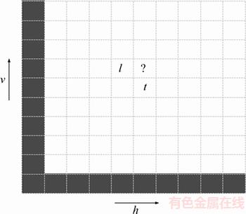
Figure 1 A two-dimensional simulation area with known left and upper boundaries

 (12)
(12)
where C is a normalizing constant and its necessity is attributed to the exclusion of unwanted transitions. Two-dimensional Markov chain can be regarded as a spatial Markov chain. The exclusion of unwanted transitions causes the small-class underestimation problem, that is, plt·k has lower value when k is a small class [18].
As shown in Figure 1, v direction actually indicates the direction from top to bottom, we choose this opposite expression to be consistent with MATLAB simulation path.
In order to overcome this problem, the full independence assumption is replaced by the conditional independence assumption as follows


 (13)
(13)
For notation convenience, the two-dimensional spatial Markov chain can be expressed as F1, F2, …, Fn with n=LN, where locations (i, j) can be indexed by a single number s=1, 2, …, n and Fs takes a value fs at cell s.
Given a cell s, its nearest known cells are sx in x direction and cell sz in z direction, which are conditionally independent. Therefore,
 (14)
(14)
Using Eq. (14) and the definition of conditional probability, we have that
 (15)
(15)
Equation (15) can also be expressed as

 (16)
(16)
Equation (15) or (16) defines the transition probability formula of the two-dimensional spatial Markov chain under the conditional independence assumption.
Methods for estimating the vertical transition probabilities in Eq. (16) have been discussed in Section 2. Similarly, the lateral transition probabilities are the entries of the lateral transition probability matrix obtained by computing the lateral transition tally matrix using Walther’s law. If we know the elongation ratios or virtual inclination of a depositional system in all directions from seismic profile, the lateral transition tally matrix can be obtained by the diagonal elements of the tally matrix of vertical transitions multiplied by the proportionality factor of the lateral and vertical elongation ratio. Detailed discussions can be found in HUANG’s research [20].
4 Three-dimensional Markov chain models
The three-dimensional Markov chain model proposed by LI et al [17] is an extension of the two-dimensional Markov chain model [16] and considers three nearest neighbors in three mutually perpendicular directions to calculate the multi-point conditional probabilities at an unknown location. The directions of three one-dimensional spatial Markov chains can be selected according to the sedimentary process.
LI et al [17] defined the three-dimensional Markov chains Zi,j,k (i=1, 2, …, L; j=1, 2, …, N; k=1, 2, …, M) by considering three one- dimensional Markov chains X1, X2, …, XL, Y1, Y2, …, YN and Z1, Z2, …, ZM together, but forcing these chains to move to equal states under the full independence assumption. The transition probabilities are given by


 (17)
(17)
where is a normalizing constant for exclusion of unwanted transitions.
The exclusion of unwanted transitions in Eq. (17) causes more serious underestimation problem than Eq. (12). For example, consider three one-dimensional Markov chains with state 1 for sandstone and state 2 for mudstone in our reservoir application. Let the transition probabilities be 0.1 from sandstone or mudstone to sandstone and 0.9 from sandstone or mudstone to mudstone. By the law of total probability, we have that the occurrence probabilities of sandstone and mudstone are 0.1 and 0.9, respectively. However, we always have that the occurrence probabilities of sandstone and mudstone are about 0.001 and 0.999 using Eq. (17), about 0.012 and 0.988 using Eq. (12) respectively. If we use the transition probability formula under the conditional independence assumption, for example, Eq. (16) in two-dimensional spatial Markov chains, we have the occurrence probability of sandstone exactly at 0.1 and that of mudstone exactly at 0.9.
To solve the underestimation problem in three- dimensional cases, we now propose the three- dimensional spatial Markov chain model. The conditional independence assumption is defined as


 (18)
(18)
Using Eq. (18) and the definition of conditional probability, we obtain the transition probability formula as follows


 (19)
(19)
where C is a normalizing constant;
 and
and represent three transition probabilities in the vertical direction, horizontal x direction and y direction, respectively; k, l, t and q all represent states in the state set Ω={1, 2, …, m}.
Equation (19) gives the transition probability expression at any unknown location with its three nearest known locations. Equation (19) is better than Eq. (17) because the former is derived under the conditional independence assumption and effectively overcomes the small-class underestimation without unwanted transitions.
5 Case studies
Firstly, we use one-dimensional Markov chain model to simulate the reservoir lithofacies of carboniferous Karashayi formation from S66 and T2 well data in the 75th block of the Tahe oilfield. Tahe Oilfield, discovered in 1990, is located on southern flank of Akekule Dome of the Tarim Basin of Xinjiang Uygur autonomous region, northwest China, with a petroliferous area of 1800 km2 [21].
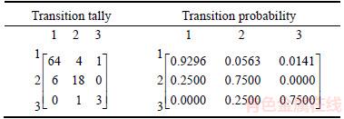
We now select two lithofacies sequences of S66 well and T2 well to illustrate the feasibility of the model. By analyzing the stratigraphic sequence diagrams of S66 and T2 wells, we find that the study area is a lowstand delta front facies sedimentary system and can be mainly divided into three kinds of lithofacies: mudstone, sandstone and conglomerate. Taking depth of 5200–5300 m as the simulation interval, and the step length in vertical direction is chosen as 1 m. The transition tally matrix and transition probability matrix in vertical direction are shown in Table 1. Since the test statistic χ2 equals 103.6125, which is greater than the threshold of the distribution it shows that the lithologic sequences have the Markov property.
Table 1 Transition tally matrix and transition probability matrix of S66 well in vertical direction
Equation (2) is used to simulate lithofacies of S66 and T2 wells by using the parameters (Table 1) estimated from S66 well data. The observed pictures and simulation results are displayed in Figure 2. Figure 2(a) shows the observed lithofacies sequence for S66 and T2 well respectively.Figure 2(b) shows the corresponding simulation results. The simulation of S66 well shows good result, while not for T2 well. This is because that our transition probabilities are estimated from S66 well, and there is not any lateral reservoir information in simulating the reservoir lithofacies of T2 well. In order to solve this problem, we need to resort to the two- and three-dimensional Markov chain models.
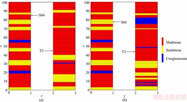
Figure 2 Observed lithofacies sequence for S66 and T2 well (a) and corresponding simulation results (b) based on one-dimensional Markov chain model
In the following, we use two-dimensional Markov chain models with the transition probabilities Eqs. (12) and (16) to simulate the reservoir lithofacies across TK667 well. The rectangular cross-section is 3000 m in length and 100 m in depth, and is discretized into grid cells with the step lengths 50 m and 1 m respectively. The left and upper boundaries (Figure 3) have been labeled by log and seismic outcrop data [22]. Transition probabilities in the vertical (z) direction can be found in Table 1, and the horizontal strike (x) direction counterparts are displayed in Table 2.
Figure 4 shows four realizations generated by Monte Carlo approach for the two dimensional Markov chain model with Eq. (12). It is clear that the occurrence frequency of mudstone (large class) is much higher than that of Figure 2, and the conglomerate (small class) in Figure 4 almost disappears. The small class (conglomerate) is underestimated, while the large class (mudstone) is overestimated. Hence the stochastic simulation, based on the independence assumption with Eq. (12), cannot correctly reproduce the reservoir lithofacies. The simulation results based on conditional independence are given in Figure 5. As we know, oil and gas resources are more likely to be distributed in conglomerate and sandstone. We find that the distribution of conglomerate always embeds in sandstone, which is in accordance with the natural phenomenon. By comparing Figure 5 with Figure 4, it is easy to see that Figure 5 is better than Figure 4, since Figure 5 has better continuity, and the small-class underestimation problem has been solved (Table 3). In addition, we find that the distribution of sandstone in Figure 4 is rather fragmented. Lithofacies patches, however, can be well represented in Figure 5.
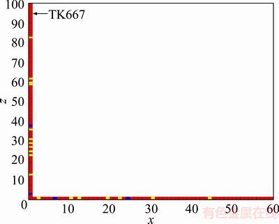
Figure 3 Rectangular cross-section to be simulated with known left and upper boundaries
Table 2 Transition tally matrix and transition probability matrix in horizontal direction
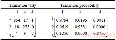
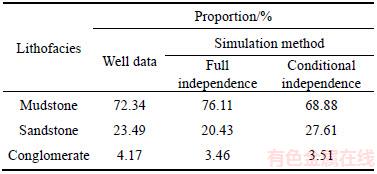
Table 3 Lithofacies proportions in well data and averaged from four simulated realizations by two- dimensional Markov chain
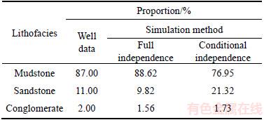
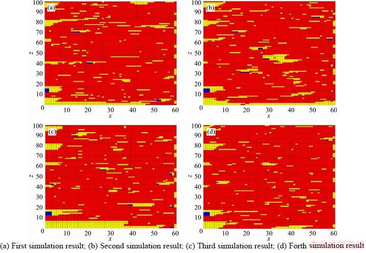
Figure 4 Four realizations of lithology stochastic simulation by two-dimensional Markov chain model with full independence assumption:
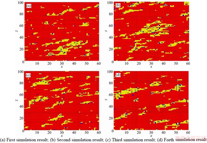
Figure 5 Four realizations of lithology stochastic simulation by two-dimensional Markov chain model with conditional independence assumption:
We have got four wells’ log data in the three-dimensional space, as shown in Figure 6. Three wells are located in the corners of this work area, another well is located inside. The distance in east-west direction of the two wells is 3000 m, and 4000 m in south–north direction, the simulated space is split into a 60×80×100 grid system, each cell is a cuboid. The results of three-dimensional simulation based on Eqs. (17) and (19) are shown in Figures 7 and 8, respectively. Obviously, the results are similar to those of the two-dimensional Markov chain model, which also suggests that the conditional independence assumption can effectively overcome the small-class underestimation problem (Table 4). And the lithology distribution under conditional independence assumption is more continuous than that of full independence assumption. We also find that sandstone distribution shows clearer patch features in Figure 8, which is in accordance with the actual reservoir construction.
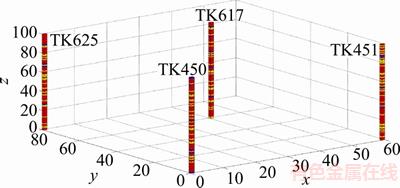
Figure 6 Three-dimensional work area with four wells (x, y and z axes indicate east–west direction, south–north direction, vertical direction respectively)
6 Conclusions
Many previous studies of Markov chain model in reservoir lithofacies stochastic simulation use the full independence assumption, however, this assumption causes the small-class underestimation problem. To solve this problem, we propose the conditional independence assumption to construct the two- and three-dimensional Markov chain model based on the idea of LI [18]. We have presented the formulas for computing the occurrence probability of each classes. Methods for determining the lateral transition probability matrix in oil-gas reservoir have also been discussed. To demonstrate the superiority of conditional independence assumption in two- and three- dimensional stochastic simulation, we use the available well data and outcrop data gathered from Tahe oilfield to estimate the lithofacies distribution in the unknown cross-section and three-dimensional work area. Simulation results indicate that, compared with full independence assumption, methods based on conditional independence assumption perform relatively better in maintaining the true composition. In addition, reservoir continuity can be well reproduced and block patches can be successfully detected by adopting the conditional independence assumption.
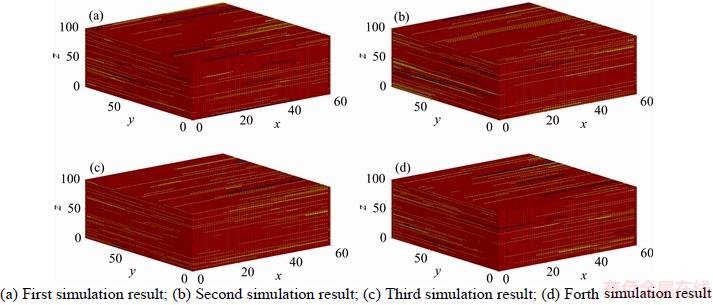
Figure 7 Four realizations of lithology stochastic simulation by three-dimensional Markov chain model with full independence assumption:

Figure 8 Four realizations of lithology stochastic simulation by three-dimensional Markov chain model with conditional independence assumption:
Table 4 Lithofacies proportions in well data and averaged from four simulated realizations by three- dimensional Markov chain
Since the petroleum geostatistics are active research areas, it is our conviction that our methods provide a useful tool for characterizing reservoir heterogeneity in petroleum engineering. Our multi-dimensional Markov chain models can also be used in other geosciences-related areas, where the task for modeling categorical random fields has long been considered as one of the most fundamental yet challenging problems.
References
[1]  M C, REMACRE A Z. The use of discrete Markov random fields in reservoir characterization [J]. Journal of Petroleum Science and Engineering, 2001, 32(2): 257–264.
[2] LIANG Y, WANG Z, GUO J. Reservoir lithology stochastic simulation based on Markov random fields [J]. Journal of Central South University, 2014, 21(9): 3610–3616.
[3] STREBELLE S. Conditional simulation of complex geological structures using multiple-point statistics [J]. Mathematical Geology, 2002, 34(1): 1–21.
[4]  O, STIEN M,
  H, FJELLVOLL B, ABRAHAMSEN P. Using multiple grids in Markov mesh facies modeling [J]. Mathematical Geosciences, 2014, 46(2): 205–225.
[5] Cao J H, Yang J C, Wang Y C, Wang D, Shi Y C. Extreme learning machine for reservoir parameter estimation in heterogeneous sandstone reservoir [J]. Mathematical Problems in Engineering, DOI: 10.1155/2015/287816.
[6] Cao R, Ma Y Z, Gomez E. Geostatistical applications in petroleum reservoir modelling [J]. Journal of the Southern African Institute of Mining and Metallurgy, 2014, 114(8): 625–631.
[7] Soleimani M, Shokri B J. 3D static reservoir modeling by geostatistical techniques used for reservoir characterization and data integration [J]. Environmental Earth Sciences, 2015, 74(2): 1403–1414.
[8] Eidsvik J, Mukerji T, Switzer P. Estimation of geological attributes from a well log: An application of hidden markov chains [J]. Mathematical Geology, 2004, 36(3): 379–397.
[9] LI Jun, XIONG Li-ping, ZHANG Li-qin, BIAN Guo-xing, LIU Jian. Facies controlled stochastic modeling based on Markov chain models [J]. Progress in Geophysics, 2010, 25(1): 298–302. (in Chinese)
[10] Carle S F, Fogg G E. Transition probability-based indicator geostatistics [J]. Mathematical Geology, 1996, 28(4): 453–476.
[11] Nikoogoftar H, Mehrgini B, Bahroudi A, Tokhmechi B. Optimization of the Markov chain for lithofacies modeling: An Iranian oil field [J]. Arabian Journal of Geosciences, 2015, 8(2): 799–808.
[12] Cao G, Kyriakidis P C, Goodchild M F. Combining spatial transition probabilities for stochastic simulation of categorical fields [J]. International Journal of Geographical Information Science, 2011, 25(11): 1773–1791.
[13] Huang X, Wang Z, Guo J. Prediction of categorical spatial data via Bayesian updating [J]. International Journal of Geographical Information Science, 2016, 30(7): 1426– 1449.
[14] VISTELIUS A B. On the question of the mechanism of formation of strata [J]. Doklady Akademii Nauk SSSR, 1949, 65(2): 191–194.
[15] Carle S F, Fogg G E. Modeling spatial variability with one and multidimensional continuous-lag Markov chains [J]. Mathematical Geology, 1997, 29(7): 891–918.
[16] Elfeki A, Dekking M. A Markov chain model for subsurface characterization: theory and applications [J]. Mathematical Geology, 2001, 33(5): 569–589.
[17] LI Jun, YANG Xiao-juan, ZHANG Xiao-long, XIONG Li-ping. Lithologic stochastic simulation based on the three-dimensional Markov chain model [J]. Acta Petrolei Sinica, 2012, 33(5): 846–853. (in Chinese)
[18] Li W. Markov chain random fields for estimation of categorical variables [J]. Mathematical Geology, 2007, 39(3): 321–335.
[19] LIU Zhen-feng, HAO Tian-yao, FANG Hui. Modeling of stochastic reservoir lithofacies with Markov chain model. Acta Petrolei Sinica, 2005, 26(5): 57–60. (in Chinese)
[20] Huang X, Wang Z, Guo J. Theoretical generalization of Markov chain random field from potential function perspective [J]. Journal of Central South University, 2016, 23(1): 189–200.
[21] Pan H, Luo M, Zhang Z, Fan Z. Lateral contrast and prediction of carboniferous reservoirs using logging data in Tahe oilfield, Xinjiang, China [J]. Journal of Earth Science, 2010, 21(4): 480–488.
[22] YANG Kai, AI Di-fei, GENG Jian-hua. A new geostatistical inversion and reservoir modeling technique constrained by well-log, crosshole and surface seismic data [J]. Chinese Journal of Geophysics, 2012,55(8): 2695–2704. (in Chinese)
(Edited by FANG Jing-hua)
中文导读
基于一到三维马尔科夫链的油气储层岩相随机模型
摘要:随机建模方法已经被广泛地应用于油气储层岩相的模拟中。然而,基于马尔科夫链的模拟技术仍然处于发展和完善中。这主要是由于在合理定义多维马尔科夫链的条件概率和水平方向上的转移概率时存在困难。本文着力解决这些问题。首先,基于完全独立假设和条件独立假设推导出了多维马尔科夫链条件概率的计算公式,并指出因为基于条件独立假设的多维马尔科夫链解决了小类过度小估计问题,所以更为合理。然后,给出了计算转移概率的方法:垂直方向上的转移概率可以通过统计井数据中的转移频数获取,水平方向上的转移概率则基于井数据和延伸率运用Walther定律估算得到。最后,运用提出的模型对中国塔河油田储层岩相的分布进行随机模拟。结果表明:与完全独立假设相比,基于条件独立假设的随机模拟结果更接近真实的岩相比例并能更好地重现岩相的空间特征。
关键词:独立性假设;马尔科夫链;储层岩相;小类过度小估计;转移概率
Foundation item: Project(2016YFB0503601) supported by the National Key Research and Development Program of China; Project(41730105) supported by the National Natural Science Foundation of China
Received date: 2016-12-12; Accepted date: 2017-01-23
Corresponding author: HUANG Xiang, PhD; Tel: +86–18390906346; E-mail: huangxiang@abchina.com; ORCID: 0000-0002- 2087-5838
Abstract: Stochastic modeling techniques have been widely applied to oil–gas reservoir lithofacies. Markov chain simulation, however, is still under development, mainly because of the difficulties in reasonably defining conditional probabilities for multi-dimensional Markov chains and determining transition probabilities for horizontal strike and dip directions. The aim of this work is to solve these problems. Firstly, the calculation formulae of conditional probabilities for multi-dimensional Markov chain models are proposed under the full independence and conditional independence assumptions. It is noted that multi-dimensional Markov models based on the conditional independence assumption are reasonable because these models avoid the small-class underestimation problem. Then, the methods for determining transition probabilities are given. The vertical transition probabilities are obtained by computing the transition frequencies from drilling data, while the horizontal transition probabilities are estimated by using well data and the elongation ratios according to Walther’s law. Finally, these models are used to simulate the reservoir lithofacies distribution of Tahe oilfield in China. The results show that the conditional independence method performs better than the full independence counterpart in maintaining the true percentage composition and reproducing lithofacies spatial features.
