J. Cent. South Univ. Technol. (2009) 16: 0125-0130

DOI: 10.1007/s11771-009-0021-7

Effective loading algorithm associated with explicit dynamic relaxation method for simulating static problems

ZHAO Chong-bin(赵崇斌)^{1, 2}, PENG Sheng-lin(彭省临)¹,LIU Liang-ming(刘亮明)¹, HOBBS B E², ORD A²

(1. Computational Geosciences Research Centre, Central South University, Changsha 410083, China;

2. CSIRO Division of Exploration and Mining, P. O. Box 1130, Bentley, WA 6102, Australia)

Key words:

numerical simulation; static systems; dynamic relaxation; loading algorithm；

1 Introduction

Due to computer memory limitations in the 20th century, the explicit dynamic relaxation method, which was initially proposed for solving static problems in structural engineering [1-3], has been widely used for solving static problems associated with geotechnical and geological systems [4-13]. Since the explicit dynamic relaxation method is a kind of explicit finite difference solver, a time-marching procedure is used to solve the equation of motion for each individual point or particle in a discretized system. The major advantage in using the explicit dynamic relaxation method is that both the global stiffness matrix and the global mass matrix are not needed and therefore, the requirement for computer memory is minimum in the process of a numerical analysis. This allows the numerical analysis of large-scale geotechnical and geological systems to be conducted in personal computers. For this particular reason, the explicit dynamic relaxation method has been used for many years [4-8], even in the well-known commercial computer packages such as the fast Lagrangian analysis of continua code (FLAC) [14] and the particle flow code (PFC) [15].

However, when the explicit dynamic relaxation method is used to solve a static problem, it is essential to artificially turn the static problem into a dynamic one by introducing an inertia term in the equation of motion for a point or particle in the system. This means that the static system, which has an equivalent wave speed of infinity, is replaced by the dynamic system of a finite wave speed. In order to avoid the assembly of the global mass and stiffness matrices, it is assumed that for a time step in the explicit dynamic relaxation method, there is no coupling between the particle deformation, which is obtained by solving the dynamic equilibrium equation (i.e. the equation of motion), and the particle force, which is obtained using the force/displacement relation (i.e. the particle-level constitutive equation), even if there is a strong nonlinearity between the particle deformation and the particle force in a real physical system. As for this assumption, it is at least required that (1) the time step be small enough so that the particle movements cannot pass physically from one particle to another within the corresponding time interval, and (2) the applied force increment, velocity increment and displacement increment to any particle be small enough so that the physical coupling between the particle deformation and the particle force in a real physical system can be reasonably neglected within a given time step. Although the above-mentioned first requirement was addressed in both FLAC [14] and PFC [15], the second requirement was often overlooked by most numerical modelers, who just simply used the com- mercial codes to produce “numerical solutions”. Thus,for an applied force in the artificial dynamic system that is simulated using the explicit dynamic relaxation method, it should be divided into many loading increments to satisfy the above-mentioned second requirement. In addition, for any particular loading increment in the artificial dynamic system that is simulated using the explicit dynamic relaxation method, it must take a large number of time steps to propagate the applied force increment throughout the whole system, which is the fundamental characteristic of a true static problem.

Keeping the above-mentioned considerations in mind, an effective loading algorithm was proposed for simulating static problems using the particle simulation method, which has been built in a two-dimensional particle flow code (i.e. PFC2D). In order to validate the proposed loading algorithm, the numerical simulation of biaxial tests is conducted to examine whether or not the numerical results from the proposed loading algorithm can reflect the fundamental behaviour of a true static system.

2 Theoretical considerations of effective loading algorithm for explicit dynamic relaxation method

The central idea behind the numerical simulation of a true static problem using the explicit dynamic relaxation method is that the true static system, which has an equivalent wave speed of infinity due to the lack of the initial term in the system, must be replaced by an artificial dynamic system of a finite wave speed. This will certainly create a theoretical issue, that is, how to use an artificial dynamic system to realistically reflect the fundamental behaviour of a true static system. In order to explain why we have such a theoretical issue, we can consider wave propagation in a one-dimensional elasto-dynamic bar system. If either a compressional wave (i.e. P-wave) or a shear wave (i.e. S-wave) is considered, the wave speed of the system is inversely proportional to the square root of the material density of the system, as described in the following formulas:

                          (1)

where  C_P and C_S are the wave speeds of the P-wave and S-wave, respectively; E and G are the elastic modulus and shear modulus of the bar material, respectively; ρ is the density of the bar material.

On the other hand, as mentioned in the introduction, one of the necessary conditions, under which the explicit dynamic relaxation method can produce meaningful results for the artificial dynamic system, requires that the time step be small enough so that the particle movements cannot pass physically from one particle to another within the corresponding time interval. This requirement results in a critical time step for the explicit dynamic relaxation method [15].

                              (2)

where  Δt_critical is the critical time step associated with the explicit dynamic relaxation method, m is the mass of the smallest particle in the system, k_n is the normal stiffness between two particles.

2.1 Motivation of proposing effective loading algorithm for explicit dynamic relaxation method

As the mass of a particle is directly proportional to the density of the particle, the critical time step associated with the explicit dynamic relaxation method is directly proportional to the square root of the particle density. From a theoretical point of view, the sufficient and necessary condition, under which the artificial dynamic system that is simulated using the explicit dynamic relaxation method can exactly represent a true static system, is that all the dynamic terms such as the inertial and damping terms must be identical to zero. Clearly, this sufficient and necessary condition can only be satisfied in the following two ways: (1) because the inertia force is directly proportional to the mass of a particle, the size of all particles used in the numerical simulation needs to be identical to zero; (2) because the dynamic energy can be damped out as the simulation time goes by, the time step needs to be large enough to enable the maximum velocity of any particle to approach zero in the artificial dynamic system. Since it is impossible to numerically simulate any system using the particle of either zero volume or zero density, the second way must be adopted when the explicit dynamic relaxation method is used to solve a true static problem. This means that for a given load increment, not only are many time steps (i.e. iterations) needed to propagate the load increment throughout the whole system, but also extra time steps (i.e. iterations) are needed to damp out the dynamic energy of the whole system.

In order to address the above mentioned theoretical issue, an effective loading algorithm needs to be developed and used in the explicit dynamic relaxation method. The effective loading algorithm must simultaneously satisfy the following three basic requirements: (1) the applied force increment, velocity increment and displacement increment to any particle must be small enough so that the physical coupling between the particle deformation and the particle force in a real physical system can be reasonably neglected within a given time step; (2) the time step is small enough so that the particle movements cannot physically pass from one particle to another within the corresponding time interval; and (3) the total number of the time step must be large enough within a loading increment so that not only can the applied force increment be propagated throughout the whole system, but also the dynamic energy can be damped out within the whole system. As a result, the whole system can be ensured to reach a static equilibrium state before another applied force increment is added to the system. It is clear that the satisfaction of the third requirement can effectively prevent any numerical errors during the current loading increment stage from propagating into the next loading increment stage. Although the numerical error at each individual loading increment stage may be very small, the propagation and accumulation of such small numerical errors from the beginning to the end of the numerical simulation may be large enough to contaminate the fundamental behaviours of a true static system.

2.2 Mathematical description of proposed effective loading algorithm

The mathematical description of the proposed loading algorithm can be expressed as follows. For an applied force in the static system, it needs to be divided into M loading increments:

                                  (3)

where  P is the applied force, ΔP_i is the ith loading force increment, and M is the total number of the loading steps.

For each loading force increment, ΔP_i, it is possible to find a solution, ΔS_i, which satisfies the following condition.

                        (4)

                            (5)

where  ΔS_ij is the solution at the jth time step due to the ith loading force increment, ΔS_ij-1 is the solution at the (j-1)th time step due to the ith loading force increment, v_ij is the particle velocity at the jth time step due to the ith loading force increment, and N_j is the total number of time steps for the ith loading force increment.

It needs to be pointed out that Eqn.(4) is used to ensure the convergence of the solution, while Eqn.(5) is used to guarantee the artificial dynamic system to reach a true static state, instead of approaching a steady state.

From the numerical analysis point of view, Eqn.(4) can be straightforwardly replaced by the following equation:

 j=N_i                   (6)

where  δ₁ is the tolerance of the solution accuracy.

Similarly, Eqn.(5) can be replaced by the following equation:

 j=N_i                          (7)

where  δ₂ is the tolerance that allows the artificial dynamic system to be approximately treated as a static system. In this regard, Eqn.(7) is called the static-system condition.

It needs to be pointed out that N_i can be determined using both the convergent condition and the static-system condition expressed by Eqns.(6) and (7) simultaneously, so that N_i may be different for different loading increments in the numerical simulation. It is the static-system condition that approximately warrants the solution of the static nature, if δ₂ is not strictly equal to zero.

Thus, the total solution S in correspondence with the applied force P can be expressed as

                                  (8)

It is noted that the total number of time step to produce the total solution S is calculated using the following formula:

                               (9)

Similarly, at the end of each loading increment, there exist the following relationships:

 j=1, 2, …, M                    (10)

 j=1, 2, …, M                   (11)

where  P_j is the total applied loading force at the end of loading increment j, and S_j is the total solution at the end of loading increment j. This indicates that at the end of a loading increment, a point of (P_j, S_j) can be obtained in the load-solution space. Therefore, at the end of loading increment M, M points can be obtained so that it is possible to link all these M points together to obtain a load-solution path in the load-solution space. Clearly, if P and S represent the applied loading force and the resulting displacement, then a force—displacement curve is obtained in the force—displacement space. Alter- natively, if P and S stand for the applied loading stress and the resulting strain respectively, then a stress—strain curve is obtained in the stress—strain space.

2.3 General steps of using proposed effective loading algorithm

If a biaxial compression test, which is simulated by a particle simulation model, is taken as an example, the general steps of using the proposed loading algorithm can be summarized as follows.

(1) For a given load increment, which needs to be applied to the boundary of a particle model, the servo- control technique [15] is used to apply the equivalent velocity or displacement to the boundary of the particle model. This means that an equivalent velocity is applied to the boundary of the particle model for several calculation time steps of the particle simulation. The number of the calculation time steps, during which the equivalent velocity needs to be applied to the boundary of the particle model, depends on the desired load increment that is applied to the boundary of the particle model. This step is called the loading step and the corresponding loading time or the number of the calculation time steps is called the loading period.

(2) After a loading period, the applied equivalent velocity is set to be zero so that the loading boundary of the particle model becomes frozen (i.e. fixed). This step is called the frozen step. During the frozen step, the particle simulation model is kept running iteratively until a static equilibrium state reaches. Therefore, the length of the frozen period depends on how quickly the particle simulation model can reach its corresponding static equilibrium state.

(3) When the particle simulation model reaches a static equilibrium state, the applied load increment such as the stress increment on the loading boundary of the particle model can be calculated so that the desired load increment is determined. At the same time, other concerned quantities such as the displacement increment and strain increment can be also determined. Thus, a point relating stress to strain in a stress—strain curve is obtained at the end of this step. For this reason, this step is called the result acquisition step.

(4) Steps 1 to 3 are repeated for every desired load increment until the final stage of the particle simulation is reached. As a result, many points relating stress to strain in a stress—strain curve are obtained at the end of the particular simulation.

(5) Finally, all the obtained points relating stress to strain are connected to generate a stress—strain curve, which should represent the true static behaviour of the particle simulation model.

3 Application examples of proposed loading algorithm

To demonstrate the applicability and usefulness of the proposed loading algorithm, the particle simulation method [9-11, 15] was used to conduct biaxial compression tests. As shown in Fig.1, two samples of different sizes are considered in the forthcoming particle simulation tests. The first test sample is of a small size of 1 m×2 m and simulated using 100 and 1 000 particles, respectively. When the small test sample is simulated using 100 particles, the minimum and maximum radii of the particles are approximately 5.45 and 3.63 cm, resulting in an average radius of 4.54 cm. However, when the small test sample is simulated using 1 000 particles, the minimum and maximum radii of the particles are approximately 1.72 cm and 1.15 cm, resulting in an average radius of 1.44 cm. On the contrary, the second test sample is of a large size of 1 km×2 km and also simulated using 100 and 1 000 particles. When the large sample consists of 100 particles, the minimum and maximum radii of the particles are approximately 54.52 and 36.35 m, respectively, resulting in an average radius of 45.43 m, while when the large sample consists of 1 000 particles, the minimum and maximum radii of the particles are approximately 17.24 and 11.49 m, respectively, resulting in an average radius of 14.37m. The initial porosity of both the small and the large test samples is set to be 17% in the particle simulation. Due to the significant size difference between the small and large test samples, the size effect of the test sample can be investigated through the particle simulation.

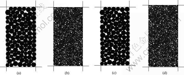
Fig.1 Initial geometrical shapes of samples used in numerical tests: (a) 1 m×2 m sample of 100 particles; (b) 1 m×2 m sample of   1 000 particles; (c) 1 km×2 km sample of 100 particles; (d) 1 km×2 km sample of 1 000 particles

The stiffness and bond strength of particles in the test sample can be determined using macroscopic mechanical properties, such as the elastic modulus, tensile and shear strength of particle materials [10-11, 15]. The analog of a two-circle contact with an elastic beam [15] demonstrated that the contact stiffness of a circular particle is only dependent on the macroscopic elastic modulus and independent of the diameter of the circular particle. The contact stiffness of a circular particle is equal to twice the macroscopic elastic modulus of the material. On the other hand, the contact bond strength of a circular particle is directly proportional to both the tensile/shear strength of the particle material and the diameter of the circular particle. Keeping the above considerations in mind, the following macroscopic mechanical properties of rock masses are used to determine the contact mechanical properties of the particle materials used in the simulation. The macroscopic elastic modulus of the particle material is 0.5 GPa, resulting in the contact stiffness (in both the normal and the tangential directions) of 1.0 GPa/m for both the small and the large test samples. The macroscopic tensile strength of the particle material is 10 MPa, while the macroscopic shear strength of the particle material is 100 MPa for both the small and the large test samples.

The robustness of the proposed loading algorithm can be examined by the simulation-solution independence of the loading rate, which is the fundamental characteristic of a true static problem. Fig.2 shows the effects of the loading rate on the curve of deviatoric stress versus axial strain for both the small and the large samples of 100 particles. It is obvious that the simulated stress—strain curve is independent of the two loading rates (i.e. P_LR=0.1 m/s and P_LR=10 m/s in this figure) in the elastic range of the test material. It can be found, from the stress—strain curve, that the simulated elastic modulus of the particle material is equal to 0.5 GPa, which is identical to the desired theoretical value of the macroscopic elastic modulus of the particle material.

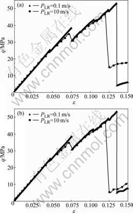
Fig.2 Effects of loading rate on curve of deviatoric stress versus axial strain (ε is axial strain and q is deviatoric stress):  (a) 1 m×2 m sample of 100 particles; (b) 1 km×2 km sample of 100 particles

As shown in Fig.3, the same conclusions can be drawn from the simulation results from using 1 000 particles in both the small and large samples. Clearly, the linear elastic modulus of either the small or the large samples is independent of the sample size, particle size and loading rate. This implies that it is potential to use a combination of the proposed loading algorithm and the explicit dynamic relaxation method to deal with multiple-length-scale static problems in particle simulations. However, compared with the particle models of 100 particles, the linear elastic ranges of the particle models of 1 000 particles are relatively large, indicating that the total number of particles, which represents the resolution of a particle model, has a significant effect on the failure pattern of the particle model. For this reason, an appropriate number of particles should be used in particle simulation models.

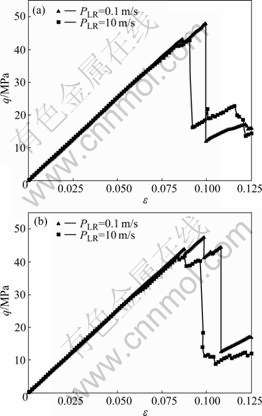
Fig.3 Effects of sample size on curve of deviatoric stress versus axial strain: (a) 1 m×2 m sample of 1 000 particles; (b) 1 km×2 km sample of 1 000 particles

Since the simulation results from the proposed loading algorithm can represent the true behaviour of a static problem, it has been demonstrated that the proposed loading algorithm associated with the explicit dynamic relaxation method is applicable, robust and useful for dealing with true static problems in a particle simulation. Thus, many static problems in engineering fields, such as crack generation problems in concrete gravity and arch dams, instability problems of rock-fill dams and high slopes, can be effectively simulated using a combination of the particle simulation method and the proposed loading algorithm.

4 Conclusions

(1) The proposed effective loading algorithm simultaneously satisfies the following three basic requirements for the particle simulation of a static problem: (a) the applied force increment, velocity increment and displacement increment to any particle are kept small enough so that the physical coupling between the particle deformation and the particle force in a real physical system can be reasonably neglected within a given time step; (b) the time step is small enough so that particle movements cannot pass physically from one particle to another within the corresponding time interval; and (c) the total number of the time step is large enough within a loading increment so that the applied force increment can be propagated throughout the whole system, ensuring that the whole system reaches a static equilibrium state before another applied force increment is added to the system.

(2) The related particle simulation results, which are obtained from the application of the proposed loading algorithm to several test samples of different sizes at different loading rates, demonstrate that a combination of the proposed loading algorithm and the explicit dynamic relaxation method can be effectively used to simulate the fundamental behaviour of a static problem in the process of the particle simulation.

References

[1] PICA A, HINTON E. Transient and pseudo-transient analysis of Mindlin plates [J]. International Journal for Numerical Methods in Engineering, 1980, 15(2): 189-208.

[2] KOBAYASHI H, TURVEY G J. On the application of a limiting process to the dynamic relaxation analysis of circular membranes, circular plates and spherical shells [J]. Computers and Structures, 1993, 48(6): 1107-1116.

[3] KADKHODAYAN M, ZHANG L C. A consistent DXDR method for elastic-plastic problems [J]. International Journal for Numerical Methods in Engineering, 1995, 38(14): 2413-2431.

[4] CUNDALL P A, STRACK O D L. A discrete numerical model for granular assemblies [J]. Geotechnique, 1979, 29(1): 47-65.

[5] CUNDALL P A. A discontinuous future for numerical modelling in geomechanics? [J]. Proceedings of the Institution of Civil Engineers: Geotechnical Engineering, 2001, 149(1): 41-47.

[6] KLERCK P A, SELLERS E J, OWEN D R J. Discrete fracture in quasi-brittle materials under compressive and tensile stress states [J]. Computer Methods in Applied Mechanics and Engineering, 2004, 193(27/29): 3035-3056.

[7] OWEN D R J, FENG Y T, DE-SOUZA-NETO E A, COTTRELL M G, WANG F, ANDRADE-PIRES F M, YU J. The modeling of multi-fracturing solids and particular media [J]. International Journal for Numerical Methods in Engineering, 2004, 60(1): 317-339.

[8] POTYONDY D O, CUNDALL P A. A bonded-particle model for rock [J]. International Journal of Rock Mechanics and Mining Sciences, 2004, 41(18): 1329-1364.

[9] ZHAO C, NISHIYAMA T, MURAKAMI A. Numerical modeling of spontaneous crack generation in brittle materials using the particle simulation method [J]. Engineering Computations, 2006, 23(5/6): 566-584.

[10] ZHAO C, HOBBS B E, ORD A, HORNBY P, PENG S, LIU L. Particle simulation of spontaneous crack generation problems in large-scale quasi-static systems [J]. International Journal for Numerical Methods in Engineering, 2007, 69(11): 2302-2329.

[11] ZHAO C, HOBBS B E, ORD A, PENG S. Particle simulation of spontaneous crack generation associated with the laccolithic type of magma intrusion processes [J]. International Journal for Numerical Methods in Engineering, 2008, 75(10): 1172-1193.

[12] SALTZER S D, POLLARD D D. Distinct element modeling of structures formed in sedimentary overburden by extensional reactivation of basement normal faults [J]. Tectonics, 1992, 11(1): 165-174.

[13] BURBIDGE D R, BRAUN J. Numerical models of the evolution of accretionary wedges and fold-and-thrust belts using the distinct- element method [J]. Geophysical Journal International, 2002, 148(3): 542-561.

[14] ITASCA C G. Fast Lagrangian analysis of continua (FLAC) [Z]. Minneapolis: Minnesota, 1995.

[15] ITASCA C G. Particle flow code in two dimensions (PFC2D) [Z]. Minneapolis: Minnesota, 1999.

Foundation item: Projects(10872219; 10672190) supported by the National Natural Science Foundation of China

Received date: 2008-06-15; Accepted date: 2008-08-01

Corresponding author: ZHAO Chong-bin, Professor; Tel: +86-731-8830843; E-mail: chongbin.zhao@iinet.net.au

(Edited by CHEN Wei-ping)