
J. Cent. South Univ. (2012) 19: 2218-2230
DOI: 10.1007/s11771-012-1266-0![]()
A novel internet traffic identification approach using wavelet packet decomposition and neural network
TAN Jun(̷��), CHEN Xing-shu(������), DU Min(����), ZHU Kai(����)
School of Computer Science, Sichuan University, Chengdu 610065, China
? Central South University Press and Springer-Verlag Berlin Heidelberg 2012
Abstract:
Internet traffic classification plays an important role in network management, and many approaches have been proposed to classify different kinds of internet traffics. A novel approach was proposed to classify network applications by optimized back-propagation (BP) neural network. Particle swarm optimization (PSO) algorithm was used to optimize the BP neural network. And in order to increase the identification performance, wavelet packet decomposition (WPD) was used to extract several hidden features from the time-frequency information of network traffic. The experimental results show that the average classification accuracy of various network applications can reach 97%. Moreover, this approach optimized by BP neural network takes 50% of the training time compared with the traditional neural network.
Key words:
1 Introduction
With the rapid development of internet technology, an increasing number of network applications have appeared. However, these applications may cause serious network and security problems. For example, network applications may take up large bandwidth, congest network access, and affect network performance greatly [1]. Also, these applications may leak the privacy of users [2]. To solve these problems, it is necessary to identify internet traffic flows effectively and accurately.
Three major approaches have been proposed to classify internet traffic flows: port based approach [3], deep packet inspection (DPI) approach [4] and statistical- based approach based on statistical characteristics of flow behavior [5-7]. However, these approaches could have potential defects. For example, current network applications may use dynamic ports to communicate with each other, and network flows among these applications cannot be easily detected by port based approach. Some applications may encrypt their data during the communication process. Therefore, the DPI approach cannot effectively identify the traffic flows of these applications.
Recently, traffic identification approaches using statistical characteristics have attracted a lot of attention, and many algorithms, such as machine learning and neural network, have been used to classify different categories of traffic flows. However, some aspects have not been considered yet. Firstly, previous work only focused on identifying TCP flows, and traffic flows using UDP protocol cannot be identified correctly. Secondly, traffic flow features are important to the identification problem, and different features may result in different classification results. Therefore, feature extraction is a key issue for traffic flow classification.
In this work, an approach was proposed to classify internet traffic flows using an optimized back- propagation (BP) neural network. This approach classified internet traffic based on the statistical characteristics of traffic flows without any port or host information, and did not need to inspect the signature of applications for privacy consideration. The contributions of this work can be summarized as follows: 1) The concepts of TCP session and UDP session were defined precisely in this approach and the proposed algorithm can classify network applications using either TCP or UDP protocol effectively. 2) The features for classification were analyzed in detail. Moreover, there was some useful information hidden in the time- frequency information of network traffic, and wavelet packet decomposition (WPD) was used to extract some useful features from network traffic. 3) BP neural network was used to classify different categories of traffic flows, and particle swarm optimization (PSO) algorithm was used to improve BP neural network, reducing the training time and increasing the recognition rate.
2 Related work
The identification of internet applications through traffic flows is important to some certain fields, such as traffic control, and quality of service. Traditionally, network applications use default port numbers to communicate with each other, and ISPs can effectively identify and classify network traffic [3]. In order to hide the traffic, some network applications have started using dynamic port numbers for communication, and some applications even use the TCP port 80 to communicate.
To solve the above problems, a new method which relies on application payload signatures was developed, which is also called deep packet inspection [4]. This approach directly compares the stored signatures to the packets from applications to accurately classify them. This method has the advantages of accuracy and real-time [8]. In addition to signature-based methods, other payload-based methods are also proposed. ACAS uses the first N bytes of payload as input to train a machine learning model to classify flows [9]. However, as some application protocols keep upgrading, new network applications emerge, also some applications even encrypt their data, making the DPI method not useful any more.
Given the shortcomings of port and signature based approaches for detecting internet traffic, many researchers classify network traffic flows based on the statistics of features of different traffic flows. KARAGIANNIS et al [10] firstly proposed the identification method based on statistical characterization, and after that there were a few methods based on the statistics of network traffic flows [11-14]. These methods collected and calculated statistics of traffic flows, such as the distribution of packet size in a flow, the duration of a flow, the interval of arrival time of each packet. ZANDER [15] firstly introduced the machine learning method to the traffic recognition problem, and used the unsupervised Bayesian learning algorithm for traffic classification. Then, a lot of internet traffic identification algorithms appeared using the algorithms in the machine learning field, such as support vector machine [16-17], decision tree algorithm [18] and neural network algorithm [19-20].
The identification methods based on the statistical characteristics of traffic flows have played a significant role in classifying different categories of network applications. However, previous studies mainly focused on the identification of TCP traffic flows, and UDP traffic flows were not considered yet [19, 21]. To the best knowledge of the authors of this work, this is the first work of UDP traffic flows identification based on the statistical characteristics of traffic flows.
3 Background
3.1 Basic concepts
A packet transmitted in the network is the manifestation of a network application. However, a single packet carries little information and has little effect on the performance of traffic identification. Therefore, a single packet should be combined with other relevant packets to form a session, and traffic flows can be classified by the form of a session.
Definition 1 (TCP session flow): Suppose host A and host B communicate with each other through TCP protocol, and their corresponding communication ports are PA and PB, respectively. Let p be a TCP session flow, and then p includes all the data packets transmitted between PA and PB. These data packets in a session should meet one and only one of the following two conditions: 1) The transmission is initialized after a SYN packet has been sent, and ended before the first FIN packet will be sent; 2) The transmission is within time t. The second condition is in case that the lifetime of a TCP session is too long.
Definition 2 (UDP session flow): Suppose host C and host D communicate with each other through UDP protocol, and their corresponding communication ports are PC and PD, respectively. Let p be a UDP session flow, and then p includes all the data packets transmitted between PC and PD within time t.
3.2 Flow features
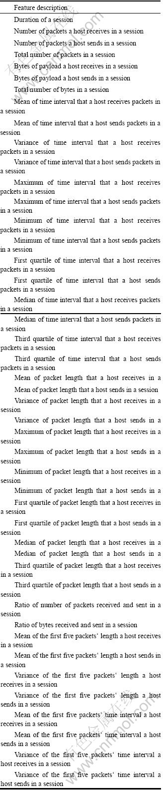
There were 246 per-flow features used for classification in Ref. [19], and most of these features could only be used for classifying TCP traffic flows, while having no use for UDP protocol. However, many more network applications use UDP protocol for transmission nowadays, such as P2P applications. Therefore, it is also important to classify UDP traffic flows. In this approach, the characteristics of many internet traffic session flows are analyzed and 45 features are selected to identify different network applications using either TCP or UDP protocols. All the features of a session are shown in Appendix A.
However, the above features can represent the differences of network behaviors only to a certain degree among different network applications, because there exists some other useful information hidden in the time-frequency information of network traffic. It is difficult to extract these useful features from the time-frequency information only using some simple transforming algorithms. So in this work, the WPD algorithm is used to extract the features hidden in the time-frequency information, and these features are defined as hidden features. WPD is used to extract hidden features from the following four traditional features: 1) Packet length that a host receives in a session; 2) Packet length that a host sends in a session; 3) Time interval that a host receives packets in a session; 4) Time interval that a host sends packets in a session.
3.3 Traffic categories
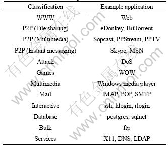
Fundamental to classification work is the idea of classes of traffic. The traffic was classified into ten categories in Ref. [19]. However, as P2P technology has been widely used in recent years, a large number of applications based on P2P technique have appeared. Many studies found that over 60% of the internet traffic nowadays comprises of P2P traffic. P2P applications have caused some serious security risks and P2P traffic identification has become a research focus in recent years. Therefore, it is necessary to divide the P2P traffic into more meticulous categories. So, internet traffic is classified into twelve categories, as listed in Table 1.
Table 1 Network traffic categories
3.4 Wavelet packet decomposition
The wavelet packet method is an expansion of classical wavelet decomposition that presents more possibilities for signal processing [22]. It includes multiple bases and different bases will result in different classification performances. In wavelet transform, signals are split into a detail and an approximation (D and A). The approximation obtained from first-level is split into new detail and approximation, and this process is repeated. Because the wavelet transform decomposes only the approximations of the signal, it may cause problems in case that some important information is located in higher frequency components. The main difference between wavelet transform and wavelet packet decomposition is that WPD splits not only approximations but also details, and WPD leads to a complete wavelet packet tree. With the use of WPD, a better frequency resolution can be obtained for the decomposed signal and it can extract more features about the signal. For a three-level decomposition, the wavelet decomposition (WD) and WPD processes are shown in Fig. 1.
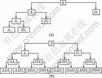
Fig. 1 Wavelet decomposition tree (a) and wavelet packet decomposition tree (b)
Let Uj,n denote the n-th (n is the frequency factor, n=0, 1, 2, ��, 2j-1) subspace of wavelet packet at the j-th scale, and ![]() is its corresponding orthonormal basis, where
is its corresponding orthonormal basis, where
![]() (1)
(1)
Parameter k is the shift factor, which satisfies with Eqs. (2) and (3):
![]() (n is even) (2)
(n is even) (2)
![]() (n is odd) (3)
(n is odd) (3)
where j, k![]() Z, n=0, 1, 2, ��, 2j-1, and h0(k) and h1(k) are a couple of quadruple mirror filters (QMF) which is irrelevant to scale band satisfies with Eq. (4):
Z, n=0, 1, 2, ��, 2j-1, and h0(k) and h1(k) are a couple of quadruple mirror filters (QMF) which is irrelevant to scale band satisfies with Eq. (4):
h1(k)=(-1)1-kh0(1-k) (4)
Sampling sequence of f(t)(f(k?t)) is directly used as the coefficient of ![]() in approximation when the scale is just enough. The coefficient of WPD at the j-th level and k-th sample can be shown as Eqs. (5) and (6) by the quadruple wavelet packet transformation:
in approximation when the scale is just enough. The coefficient of WPD at the j-th level and k-th sample can be shown as Eqs. (5) and (6) by the quadruple wavelet packet transformation:
![]() (n is even) (5)
(n is even) (5)
![]() (n is odd) (6)
(n is odd) (6)
The decomposition coefficient of the j-th level can be obtained by the (j-1)-th level, finally we can get the coefficients of all levels through sequential analogy [23].
For example, a signal S is decomposed by wavelet packet of L layers, and the signals of each sub-band are denoted as Sj,k (j=1, 2, ��, L; k=0, 1, 2, ��, 2j-1). Xj,k= ![]() is the corresponding coefficients of WPD for Sj,k, and here the N is the number of coefficients of sub-band Sj,k. Suppose the maximum modulus of coefficient of Sj,k is
is the corresponding coefficients of WPD for Sj,k, and here the N is the number of coefficients of sub-band Sj,k. Suppose the maximum modulus of coefficient of Sj,k is ![]() Then, the maximum modulus of coefficient of each layer is
Then, the maximum modulus of coefficient of each layer is
![]()
(j=1, 2, ��, L; k=0, 1, 2, ��, 2j-1) (7)
The wavelet energy is the sum of square of detailed wavelet transform coefficients. The energy of wavelet coefficient varies over different scales depending on the input signals.
The energy of each coefficient can be defined as
![]()
![]() (8)
(8)
And the energy of Sj,k can be defined as
![]() (9)
(9)
A signal can be expanded in different ways and the number of binary sub trees may be very large. It is necessary to find an optimal decomposition by using a convenient algorithm. Entropy is a common method in many fields, especially in signal processing applications. Entropy indicates the amount of information which is stored in observed signal. One of the most effective entropy types is Shannon.
According to Shannon, the entropy of Sj,k can be defined as
![]()
![]() (10)
(10)
Then, the minimum sub-band entropy of each layer is
![]()
![]() (11)
(11)
3.5 BP neural network
Artificial neural networks (ANNs), due to their excellent ability of non-linear mapping, generalization, self-organization and self-learning, have been proved to be of widespread utility in engineering and are steadily advancing into new areas. The BP neural network is a widely used supervised neural network model [24-26]. A typical BP neural network consists of one input layer, one or more hidden layers and one output layer. Each layer comprises several nodes, called neurons. In a standard BP structure, the neurons on two adjacent layers are fully connected. The total numbers of neurons in the input and output layers are determined according to the dimensions of input and output vectors in the problem. However, the appropriate number of hidden layers and neurons on each layer cannot be known in advance. Moreover, choosing an appropriate network structure is very important but difficult, since a network smaller than needed may be unable to provide good performance owing to its limited information processing power and a network larger than needed may have redundant information among its connections. The training of a BP neural network to a specific problem includes the feed-forward and back-propagation processes. Three stages include: feed-forward of the input training pattern, calculation and back-propagation of the associated error, and weight and bias adjustment. These processes are utilized repeatedly until the mean square error associated with the training samples reaches a specific precision. A typical three-layer BP neural network is shown in Fig. 2.
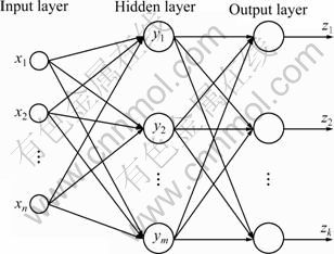
Fig. 2 Typical BP neural network model
Assume a three-layer BP neural network has n inputs, m hidden nodes and k outputs. The weight between input node xi (1��i��n) and hidden node yj (1��i��m) is defined as ��ji, and the weight between the hidden node yj and output node zl (1��l��k) is defined as vlj. The bias of hidden node yj is ��j, and the bias of output node zl is ��l. Each neuron in the hidden layer uses Sigmoid function f(x) as its threshold function, and each neuron in the output layer uses Purelin function p(x) as its threshold function. Therefore, the neuron output of hidden node yj and output node zl can be expressed as
![]() (12)
(12)
![]() (13)
(13)
The threshold functions are defined as
![]() (14)
(14)
![]() (15)
(15)
Assume that there are H samples denoted as X={X1, X2, ��, Xi, ��, XH}, and each sample Xi in set X is a n-dimensional feature vector. Let T={T1, T2, ��, Ti, ��, TH} be the corresponding output of set X. For each output, Ti=[t1, t2, ��, tj, ��, tk] is a k-dimensional class vector. If the target class for a given sample is j (1��j��k), then we have tj=1, otherwise tj=0. Define zij as the j-th actual neuron output for the input training sample Xi at the output layer, while tij is its desired response. The mean square error function for this neural network would be described as
![]() (16)
(16)
In this internet traffic identification problem, the input sample is the statistics of features of a session, the number of input nodes is the feature used for classification, and in this work, we use two kinds of features: one is the traditional features listed in Appendix A, and the other one is the hidden features extracted by WPD. The output represents the class that the input sample belongs to, so the number of output nodes is 12 as described in Table 1. Since a three-layer feed forward artificial neural network can approximate any nonlinear continuous function to an arbitrary accuracy, in this approach, the three-layer neural network was adopted for classification.
3.6 Particle swarm optimization
PSO is an evolutionary computation technique developed by KENNEDY and EBERHART [27] in 1995, which searches for the best solution by simulating the movement and flocking of birds. PSO is an optimization tool, providing a population-based search procedure in which individuals called particles change their positions with time. In a PSO system, the group is a community composed of all particles, and all particles fly around in a multi-dimensional search space. Each particle flies with a certain velocity and finds the global best position after some iteration. At every iteration period, each particle adjusts its velocity vector based on its momentum and the influence of its best position in history as well as the best position of all particles, then a new position is computed by the velocity and its position in the last iteration.
Suppose that the dimension for a searching space is Q, the total number of particles is P, the population is presented as X=(x1, ��, xi, ��, xP)T, and the position of the i-th particle is described as vector xi=(xi1, xi2, ��, xiQ)T. The velocity of the i-th particle is presented as vector vi=(vi1, vi2, ��, viQ)T, the best position of this particle being searched until now is denoted as pi=(pi1, pi2, ��, piQ)T, and the best position of the whole population being searched until now is denoted as pg= (pg1, pg2, ��, pgQ)T. The rule of adjusting the velocity and position of a particle is described as
![]() (17)
(17)
![]() (18)
(18)
where i(=1, 2, ��, P) represents the number of particles; d(=1, 2, ��, Q) represents the searching space of this problem; t is the current evolution generation; r1 and r2 are random numbers between 0 and 1; c1 and c2 are the acceleration constants with positive values; w is the inertia weight. The general steps involved in PSO are illustrated as follows [28-29]:
Algorithm 1: Particle swarm optimization
Step 1: Provide a population of particles with random position xi and velocity vi for each particle i;
Step 2: If a stopping criterion is not satisfied, then
1) Evaluate the fitness value of each particle and then update the current best position pi and fitness value pbest;
2) Compare the fitness values pbest of all particles and then update the current global best position pg and the fitness value gbest;
3) Update the velocity and position of each particle according to Eqs. (17) and (18);
End if.
4 Feature extraction and classification algorithm
4.1 Approach overview
The training and testing processes of the identification system are presented as follows:
1) Capture and reorganize all the packets into traffic session flows according to Definition 1 and Definition 2, and divide the traffic flows into training set and testing set;
2) Calculate the feature statistics of traffic flows according to Appendix A;
3) Extract the hidden feature statistics of traffic flows by wavelet packet decomposition;
4) Preprocess the statistics of features using normalization method;
5) Train the data in the training set using the optimized BP neural network algorithm proposed in this approach and then the corresponding neural networks are obtained, which are used for classifying the data in testing set later.
As we will classify network applications using either TCP or UDP protocol in this approach, two neural networks are used for training and classifying TCP and UDP traffic flows, respectively. One is for TCP flows and the other is for UDP. For a traffic session flow to be classified, firstly check it if it is TCP or UDP protocol, and then classify it using the corresponding BP neural network. The system overview is presented in Fig. 3.
4.2 Feature extraction by WPD
WPD is an effective method for feature extraction. It takes full advantages of time-frequency information, and can highlight some features which are hard to observe in time-domain signal. It can be seen from Fig. 1(b) that there are many choices to reconstruct a signal according to its decomposition tree of WPD. Different bases will result in different performances. Figure 4 shows two possible scenarios of best WPD tree, the grey nodes are the best bases.
The best basis contains primary information of original signal, and in some cases we can use best basis to construct feature vector. However, as shown in Fig. 4, the network traffic is rather complicated, and the structure of best WPD tree is uncertain even for the same kind of flow-signal of different flows. It is difficult to construct the standard feature vector, as the dimension of the vector is uncertain, and the meaning of the same component in different vectors might be inconsistent, which is an essential requirement for a classifier. To solve this problem, a new feature extraction algorithm of flow signal is presented in this work.
Algorithm 2: Hidden features extracted based on WPD
Step 1: Select a wavelet function and specify the decomposition Layer as L;
Step 2: Decompose the signal to the specified layer using the selected wavelet function and obtain the decomposition coefficients;
Step 3: Obtain the maximum modulus of coefficient Xmax of each layer;
Step 4: Calculate the entropy of each sub-band;
Step 5: Calculate the minimum sub-band entropy ��min of each layer;
Step 6: Construct the feature vector of flow signal S as
AS(c)=( ��min(1), Xmax(1), ��, ��min(L), Xmin(L))
In Algorithm 2, we extract the best entropy and maximum modulus of coefficients of each layer, which could contain important information of the original signal and these features have the advantages of losing no information. Another key stage in wavelet packet decomposition is the selection of wavelet function. In our investigation, we select Daubechies wavelet by comparing and computing different wavelet bases. The reason is that it possesses some fine characteristics: orthogonality, losslessness, power complementary, biorthogonality, and compact support. We set the layer L as 3 in this work, so the dimension of the feature vector obtained is 2��3=6.
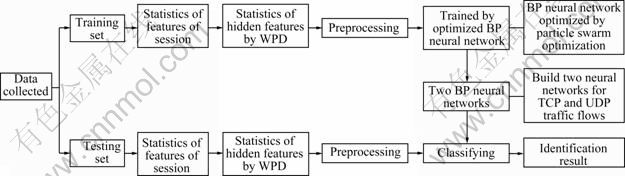
Fig 3 System overview
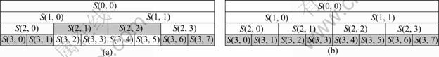
Fig. 4 Two best WPD trees: (a) Best WPD tree 1; (b) Best WPD tree 2
4.3 BP neural network optimized by PSO
The BP neural network optimizes the target function using the gradient descent method, and the target function is the mean square error of the actual outputs and the desired outputs. However, there exists four main defects [30]: 1) The calculation results may fall into local minimum values; 2) The performance of neural network is affected by the choice of topology and size, and different numbers of hidden nodes may lead to different results; 3) The results may also be affected by the initial selection of weights, and if the initial sets of weights are not selected properly, the optimization solution could get trapped into a local optimum; 4) The training speed of the traditional BP neural network is generally slow.
The topology of a neural network has great influence on the performance, but the determination of the number of hidden nodes is usually solved by experience currently [19], resulting in the generalization ability of the neural network not guaranteed. If some conditions change, the structure will be adjusted manually. The convergence speed of PSO algorithm is fast, and the population-based property ensures PSO algorithm to be less likely to fall into a local minimum, thus it is suitable for global search. So, a combination of PSO and BP algorithm is proposed in this work, and the defects of BP algorithm are offset by the characteristics of PSO. The PSO is deployed to optimize the initial weights, and bias of the neural network.
The methodology of this algorithm is described as follows: First of all, a PSO is used to optimize the initial weights and bias of the neural network; and when the PSO terminates, the initial weights and bias are determined, then the traditional gradient descent method is applied to optimize the neural network. This process is presented in Fig. 5.
In order to optimize the initial weights and bias, and in the calculation of the initial weights and bias for a neural network whose number of hidden nodes has been set, the encoding is presented as
![]()
![]() (19)
(19)
where n is the number of input nodes, X is the number of hidden nodes, and k is the number of output nodes.
In the optimization process of the PSO, the fitness value is determined by the mean square error (MSE) in Eq. (16). The smaller the MSE is, the better the performance of the neural network is. The fitness function is presented by
![]() (20)
(20)
where EMS is the mean square error mentioned in Eq. (16). The proposed algorithm is described as follows:
Algorithm 3: BP neural network optimized by PSO
Generation �� 1
while generation �� maxgeneration do
j �� 1
while j �� population_size do
Evaluate the fitness of each particle as f
if f is better than the current best fitness value then
replace this particle��s best fitness with f and save the current position
end if
if f is better than the best fitness value of all particles then
replace the population��s best fitness with f and save the current position
end if
end while
update each particle according to Eqs. (17) and (18)
end while
Get the initial weights and bias
Optimize the BP neural network using the traditional gradient descent method
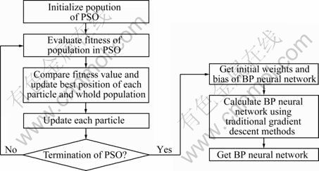
Fig. 5 Approach flowchart
5 Experiment
5.1 Experiment design
The data collection environment is shown in Fig. 6.
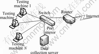
Fig. 6 Data collection environment
In a data collection process, all the testing machines are running network applications belonging to one of the above categories listed in Table 1, so all the traffic flows collected at each time belong to only one specific class, and these flows are collected by the data collection server through port mirroring method. Total up to 40 000 flows are collected for a specific traffic category. Following these steps, all the traffic flows belonging to the 12 classes listed in Table 1 are collected, so that one data set contains 12��40 000 traffic flows.
In order to verify the effectiveness of the method proposed in this work, two separate data sets were collected. The first data set was collected from January 18th, 2010 to January 24th, 2010, the second data set was collected from September 20th, 2010 to September 26th, 2010, and these two data sets are separated by eight months. They are denoted as set 1 and set 2, respectively.
The experiment process is described as follows: 50% of the data were randomly chosen from set 1 as the training data, and the data in set 2 were used for testing. This experiment was repeated for ten times using different randomly chosen training sets of the same size, and the mean and standard deviation across the repeated experiments were calculated.
5.2 Hidden feature extraction based on WPD
In order to increase the identification performance, WPD is used to extract some useful features from the time-frequency information. And in this work, four kinds of flow signals are analyzed in detail: 1) Packet length that a host receives in a session; 2) Packet length that a host sends in a session; 3) Time interval that a host receives packets in a session; 4) Time interval that a host sends packets in a session.
On the whole, the oscillograms of different network applications have some differences, which make it possible to classify network traffic using the features extracted from the time-frequency information. In our experiments, we use the Daubechies wavelet for feature extraction, and the number of decomposition layer is 3. The hidden features of the above four kinds of flow signals are extracted by Algorithm 2. And six hidden features are extracted from one traditional feature as described in Algorithm 2. Therefore, the total number of hidden features obtained is 6��4=24.
The value of hidden features of each network application is shown in Figs. 7 and 8. Figure 7 shows the minimum sub-band entropies and the maximum modulus of the coefficients of the three layers of the oscillograms of time interval that a host sends packets in a TCP session flow, and Fig. 8 shows the same kinds of values of UDP session flow. There are eleven kinds of network traffic using TCP protocol except the Attack protocol, since we only send UDP packets in our DDoS Attack experiment. There are only four kinds of network traffic using UDP protocol, since WWW and other applications only use TCP protocol. The X axis represents the network applications, and the Y axis represents the hidden features extracted by WPD. Six hidden features are extracted from one traditional feature as described in Algorithm 2. In Fig. 7, corresponding to the 1-11, the eleven kinds of network traffics are as follows: Bulk, DataBase, Games, Interactive, Mail, Multimedia, P2P FileSharing, P2P IM, P2P Multimedia, Services, and WWW. In Fig. 8, corresponding to 1-4, four kinds of network traffics are as follows: Attack, P2P FileSharing, Games, and P2P Multimedia.
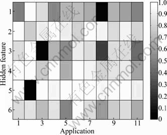
Fig. 7 Hidden features extracted by WPD of TCP protocol
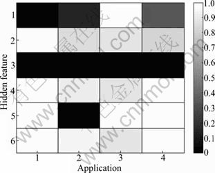
Fig. 8 Hidden features extracted by WPD of UDP protocol
It can be seen from two figures that there exist some obvious differences among different network applications, and these hidden features are used to increase the identification performance.
5.3 Choosing architecture
It should be decided what kind of network architecture is most applicable in this problem. One hidden layer is used in our BP neural network, and it is necessary to calculate the best suitable number of hidden layer nodes. Here, the average identification rate is also used for the decision: We trained the neural networks with different structures on a subset of the data, and calculated the average identification rate on another set of data. For simplicity, networks with 1-50 nodes in the hidden layer are considered. As we had mentioned before, we would classify both TCP and UDP traffic flows, and built two neural networks respectively. Therefore, two experiments are used to determine the numbers of the two neural networks. The average identification rates for TCP and UDP traffic with different numbers are shown in Figs. 9(a) and 9(b), respectively.
As seen from Fig. 9(a) that when the number of hidden layer nodes is 17, the average identification rate becomes steady, and there is no obvious increase of the average identification rate. Fewer nodes will take less time to compute, therefore, for TCP traffic classification, we set the number of hidden layer as 17. From Fig. 9(b), it can be seen that when the number of hidden layer nodes is 23, the average identification rate becomes steady, so the number was set as 23 for UDP traffic classification.
5.4 Determination of interval time in traffic session
As described in Definition 1 and Definition 2, the TCP and UDP session flows include all the packets transmitted within time t, and the determination of t has great influence on the identification rate as well as the computation performance. If t is too small, the number of packets collected is also too small to form the information which has the property of statistical characteristics. If t is too large, the packets collected will take up a significant amount of system resources. We tested the value of t from 20 s to 300 s, and we also did two separate experiments. In the first experiment, we only used the traditional features listed in Appendix A, and in the second one we used the traditional features as well as the hidden features extracted by WPD as mentioned before. Moreover, the TCP and UDP are two different network protocols and they are defined separately, so we measured the interval time of TCP and UDP protocols respectively. The average identification rate of TCP sessions is presented in Fig. 10(a), and the average identification rate of UDP sessions is presented in Fig. 10(b).
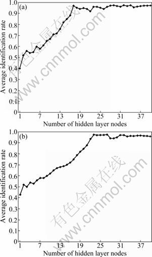
Fig. 9 Average identification rates of different hidden numbers for TCP traffic (a) and UDP traffic (b)
Through experiments, it can be seen that in the test of TCP session interval time, while only using the traditional features listed in Appendix A, if t is larger than 100 s, the identification rate becomes steady; however, while using the traditional features with the hidden features, if t exceeds 60 s, the identification rate becomes steady, and when t is 40 s, the average identification rate of TCP traffic exceeds 90%, about 30% higher than that only using the traditional features. Similarly, for UDP traffic experiments, the time is 80 s and 60 s for two kinds of features, respectively.
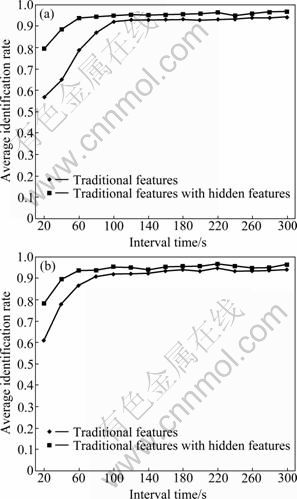
Fig. 10 Identification rate of TCP session (a) and UDP session (b) using different time t
The experiments demonstrate that according to the Definition 1 and Definition 2, network traffic can be classified within time t; however, if we only use the traditional features, it takes longer time to reach a high identification accuracy. So, with the use of hidden features, we have decreased the time. In this way, this scheme can use the information of network traffic more effectively and achieves better real-time performance.
5.5 Identification rate comparison
According to the algorithm proposed in Section 4.3, when the numbers of hidden nodes are 17 and 23 for TCP and UDP neural networks, respectively, the average identification rates for the entire internet traffic flows are the highest. The false positive (FP) and false negative (FN) of each class are listed in Table 2.
Table 2 False positives and false negatives of all classes
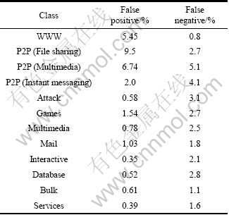
From Table 2, it can be seen that the FPs and FNs of some traditional network applications are smaller than those of newly emerging applications. For instance, we have smaller FPs and FNs of the Mail, Bulk and some other applications; however, the FPs and FNs of P2P applications are not so good. The reason for this situation is that, P2P technology is a kind of complex network applications, and it uses both TCP and UDP traffic flows for communication. Moreover, P2P networking is a distributed application architecture where partitions tasks or workloads between peers, and peers are both suppliers and consumers of resources, in contrast to the traditional client-server model where only servers supply, and clients consume. For these reasons, P2P applications have a lower identification rates than those traditional network applications.
The average identification rate of the optimized BP algorithm, the traditional BP algorithm and the Bayesian neural network in Ref. [19] are listed in Table 3.
Besides choosing 50% of the data in set 1, we also choose 0.1%, 1% and 10% of the data in set 1 for testing. As seen from Table 4, the identification rate of optimized BP algorithm increases by 14.3% compared with the traditional algorithm, proving that the optimized algorithm is effective for improving the recognition rate. Compared with the method in Ref. [19], the method in this approach also increases the recognition rate, and more importantly, the method in this work can classify both TCP and UDP traffic flows, while the method in Ref. [19] could only deal with TCP traffic flows. Therefore, the proposed method is more competitive.
Table 3 Identification rates of all algorithms
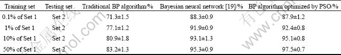
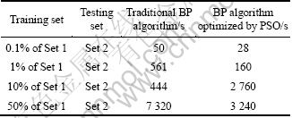
Table 4 Training time of different algorithms
5.6 Training time comparison
The speed of BP neural network trained by PSO and traditional gradient descent method is faster than that only using the gradient descent method. We set the training accuracy of the whole algorithm as 1��10-4, and set 1��10-2 as the training accuracy of PSO, while the results of PSO algorithm are the initial weights and bias of the following BP algorithm. The numbers of hidden nodes are 17 and 23 respectively for TCP and UDP neural networks as calculated in Section 5.3.
The training time of the PSO optimized BP algorithm and the traditional BP algorithm are listed in Table 4. As we can see from Table 4, the training speed of the optimized BP algorithm is faster than that of the traditional BP algorithm. The main reason for this improvement is that the PSO optimized BP algorithm accelerates the convergence rate, which can also reduce the training time.
6 Conclusions
1) The optimization of traditional BP neural network algorithm in this work improves the identification rate as well as the training speed. The experimental results demonstrate that the proposed algorithm can classify internet traffic at a high rate. Also by the wavelet packet decomposition algorithm, some useful features are extracted from the time-frequency information, making this approach classify network traffic much faster.
2) However, there are also some weaknesses in this work. Firstly, there are still 45+24=69 features calculated, and calculating so many features still takes a lot of time. Secondly, the port and signature based approaches still have effects for some network applications. If these two methods can be combined with the statistical characteristics of traffic flows approach, the identification performance will get better. Therefore, in the future work, we will select the best feature subset for classification based on some intelligent algorithm, thus reducing the training time while not affecting the identification rate. Also, we will consider a multilayer classification model which combines the three main approaches for Internet traffic classification.
Appendix A
All the features of a session are described below:
References
[1] AZZOUNA N B, GUILLEMIN F. Impact of peer-to-peer applications on wide area network traffic [C]// Proc of IEEE Global Telecommunications Conference. Texas: IEEE, 2004: 1544-1548.
[2] KIM J T, PARK H K, PAIK E H. Security issues in peer-to-peer systems [C]// The 7th International Conference on Advanced Communications Technology. Phoenix Park: IEEE, 2005: 1059- 1063.
[3] SEN S, WANG J. Analyzing peer-to-peer traffic across large networks [J]. IEEE Trans on Networking, 2004, 2(2): 219-231.
[4] SEN S, SPATSCHECK O, WANG Dong-mei. Accurate, scalable in-network identification of P2P traffic using application signatures [C]// Proceedings of ACM WWW��04. New York: ACM, 2004: 512-521.
[5] ERMAN J, MAHANTI A, ARLITT M, COHEN I, WILLIAMSON C. Semi-supervised network traffic classification [C]// Proceedings of the ACM SIGMETRICS, New York: ACM, 2007: 369-370.
[6] ZANDER S, NGUYEN T, ARMITAGE G. Self-learning IP traffic classification based on statistical flow characteristics [J]. Passive and Active Network Measurement, 2005, 3431: 325-328.
[7] MOORE A W, ZUEV D. Internet traffic classification using bayesian analysis techniques [C]// Proceedings of the ACM SIGMETRICS. 2005: 50-60.
[8] MOORE A W, PAPAGIANNAKI K. Towards the accurate identification of network applications [C]// Passive and Active Measurements Workshop. Boston, MA, USA, Springer Press, 2005: 41-54.
[9] HAFFNER P, SEN S, SPATSCHECK O, WANG Dong-mei. ACAS: automated construction of application signatures [C]// Proceedings of the 2005 ACM SIGCOMM Workshop on Mining Network Data. ACM, New York, 2005: 192-202.
[10] KARAGIANNIS T, BROIDO A, FALOUTSOS M, CLAFFY K. Transport layer identification of P2P traffic [C]// Proceedings of the 4th ACM SIGCOMM conference on Internet Measurement. Sicily, USA: ACM, 2004: 121-134.
[11] XU Ke, ZHANG Ming, YE Ming-jiang, CHIU Dah-ming, WU Jian-ping. Identify P2P traffic by inspecting data transfer behavior [J]. Computer Communications, 2010(33): 1141-1150.
[12] FILHO R H, CARMO M F F D, MAIA J E B, JUNIOR G P S. An Internet traffic classification methodology based on statistical discriminators [C]// Network Operations and Management Symposium, Salvador: IEEE, 2008: 907-910.
[13] WILLIAMS N, ZANDER S, ARMITAGE G. A preliminary performance comparison of five machine learning algorithms for practical IP traffic flow classification [J]. SIGCOMM Computer Communication Review, 2006, 36(5): 5-16.
[14] LU X, DUAN H, LI X. Identification of P2P traffic based on the content redistribution characteristic [J]. Communications and Information Technologies, 2007: 596-601.
[15] ZANDER S, NGUYEN T, ARMITAGE G. Automated traffic classification and application identification using machine learning [C]// Proceedings of the IEEE Conference on Local Computer Networks 30th Anniversary. Sydney, NSW: IEEE Press, 2005: 250-257.
[16] ESTE A, GRINGOLI F, SALGARELLI L. Support vector machines for TCP traffic classification [J]. Computer Networks, 2009, 53(14): 2476-2490.
[17] LI Zhu, YUAN Rui-xi, GUAN Xiao-hong. Accurate classification of the internet traffic based on the SVM method [C]// IEEE International Conference on Communications. Glasgow: IEEE Press, 2007: 1373-1378.
[18] RAAHEMI B, ZHONG Wei-cai, LIU Jing. Peer-to-peer traffic identification by mining IP layer data streams using concept-adapting very fast decision tree [C]// Proc of the 20th IEEE International Conference on Tools with Artificial Intelligence. Dayton, USA: IEEE Press, 2008: 525-532.
[19] AULD T, MOORE A W, GULL S F. Bayesian neural networks for internet traffic classification [J]. IEEE Transaction on Neural Networks, 2007, 18(1): 223-239.
[20] SUN Run-yuan, YANG Bo, PENG Li-zhi, CHEN Zhen-xiang, ZHANG Lei, JING Shan. Traffic classification using probabilistic neural networks [C]// Sixth International Conference on Natural Computation (ICNC). Yantai: IEEE Press, 2010: 1914-1919.
[21] CALLADO A, KELNER J, SADOK D, KAMIENSKI C A, FERNANDES S. Better network traffic identification through the independent combination of techniques [J]. Journal of Network and Computer Applications, 2010, 33(4): 433-446.
[22] EKICI S, YILDIRIM S, POYRAZ M. Energy and entropy-based feature extraction for locating fault on transmission lines by using neural network and wavelet packet decomposition [J]. Expert Systems with Applications, 2007, 34(4): 2937-2944.
[23] WU Ting, YAN Guo-zheng, YANG Bang-hua, SUN Hong. EEG feature extraction based on wavelet packet decomposition for brain computer interface [J]. Measurement, 2007, 41(6): 618-625.
[24] SEDKI A, OUAZAR D, MAZOUDI E E. Evolving neural network using real coded genetic algorithm for daily rainfall-runoff forecasting [J]. Expert Systems with Applications, 2009, 36(3): 4523-4527.
[25] LIU Zheng-jun, LIU Ai-xia, WANG Chang-yao, NIU Zheng. Evolving neural network using read coded genetic algorithm (GA) for multispectral image classification [J]. Future Generation Computer Systems 2004, 20(7): 1119-1129.
[26] ZHANG Jing-ru, ZHANG Jun, LOK Tat-ming, LYU M R. A hybrid particle swarm optimization-back-propagation algorithm for feedforward neural network training [J]. Applied Mathematics and Computation, 2007, 185(2): 1026-1037.
[27] KENNEDY J, EBERHART R. Particle swarm optimization [C]// Proceeding of IEEE International Conference on Neural Networks. Perth: IEEE Press, 1995: 1942-1947.
[28] LI Te-sheng, HSU Chih-ming. Parameter optimization of sub-35 nm contact-hole fabrication using particle swarm optimization approach [J]. Expert Systems with Applications, 2010, 37(1): 878-885.
[29] LIN Cheng-jian, WANG Jun-guo, LEE Chi-yung. Pattern recognition using neural-fuzzy networks based on improved particle swarm optimization [J]. Expert Systems with Applications 2009, 36(3): 5402-5410.
[30] YU Shi-wei, ZHU Ke-jun, DIAO Feng-qin. A dynamic all parameters adaptive BP neural networks model and its application on oil reservoir prediction [J]. Applied Mathematics and Computation, 2008, 195(1): 66-75.
(Edited by DENG L��-xiang)
Foundation item: Project(2007CB311106) supported by National Key Basic Research Program of China; Project(NEUL20090101) supported by the Foundation of National Information Control Laboratory of China
Received date: 2011-07-04; Accepted date: 2011-10-21
Corresponding author: CHEN Xing-shu, Professor, PhD; Tel: +86-13981857689; E-mail: chenxs@scu.edu.cn
Abstract: Internet traffic classification plays an important role in network management, and many approaches have been proposed to classify different kinds of internet traffics. A novel approach was proposed to classify network applications by optimized back-propagation (BP) neural network. Particle swarm optimization (PSO) algorithm was used to optimize the BP neural network. And in order to increase the identification performance, wavelet packet decomposition (WPD) was used to extract several hidden features from the time-frequency information of network traffic. The experimental results show that the average classification accuracy of various network applications can reach 97%. Moreover, this approach optimized by BP neural network takes 50% of the training time compared with the traditional neural network.
