
J. Cent. South Univ. (2017) 24: 2532-2541
DOI: https://doi.org/10.1007/s11771-017-3666-7

Structural reliability analysis using a hybrid HDMR-ANN method
Bhaw Nath Jha, LI Hong-shuang(���˫)
Key Laboratory of Fundamental Science for National Defense-Advanced Design Technology of Flight Vehicles, Nanjing University of Aeronautics and Astronautics, Nanjing 210016, China
 Central South University Press and Springer-Verlag GmbH Germany, part of Springer Nature 2017
Abstract:
A new hybrid method is proposed to estimate the failure probability of a structure subject to random parameters. The high dimensional model representation (HDMR) combined with artificial neural network (ANN) is used to approximate implicit limit state functions in structural reliability analysis. HDMR facilitates the lower dimensional approximation of the original limit states function. For evaluating the failure probability, a first-order HDMR approximation is constructed by deploying sampling points along each random variable axis and hence obtaining the structural responses. To reduce the computational effort of the evaluation of limit state function, an ANN surrogate is trained based on the sampling points from HDMR. The component of the approximated function in HDMR can be regarded as the input of the ANN and the response of limit state function can be regarded as the target for training an ANN surrogate. This trained ANN surrogate is used to obtain structural outputs instead of directly calling the numerical model of a structure. After generating the ANN surrogate, Monte Carlo simulation (MCS) is performed to obtain the failure probability, based on the trained ANN surrogate. Three numerical examples are used to illustrate the accuracy and efficiency of the proposed method.
Key words:
1 Introduction
Many sources of uncertainties are inherent in structural and mechanical design. Therefore, the parameters of the loading and the load carrying capacity of structures are not deterministic quantities. They are uncertain variables and thus absolute safety cannot be achieved. This means that there is always a failure probability for a structure or mechanical system if uncertainties are modeled by random variables. The reliability of a structure or system is its ability to fulfill its design purposes for some specified design lifetime. In other words, reliability is the probability that a structure or system will not fail to perform its intended function [1, 2]. Here, failure not only means the catastrophic failure of a system but also is used to indicate the inability of a structure to perform the desired function.
One of the main purposes of structural reliability analysis is the evaluation of failure probability for a given limit state function g(x) [1, 2]. Due to the nonlinearity and implicit nature of limit state function, difficulties arise in calculating structural reliability. The first order or second-order reliability method (FORM/SORM) in conjunction with detailed finite element (FE) modeling can be used to calculate the probability of failure [3]. However, FORM/SORM may provide correct results only if the most probable point (MPP) is accurately and efficiently found. The searching process of MPP can be performed by a gradient based optimization algorithms. However, the occurrence of multiple MPP or highly non-linear limit state function can give rise to large error in function approximation and also increase the computational effort. PENMETSA and GRANDHI [4] proposed a two-point adaptive non-linear approximation to construct the approximate limit state function and used fast Fourier transformation (FFT) for the failure probability estimation. WU and TORNG [5] suggested a quadratic approximation of the limit state function at the most MPP and adopted FFT to estimate the failure probability. Since the calculation of failure probability is dependent on MPP, high order function approximation maybe better than the quadratic approximation. The above structural reliability methods belong to the category of analytical methods. In this category, there is a group of methods which do not require the searching of MPP. They are moment methods developed by ZHAO et al [6�C8]. However, the applicable ranges of moment methods have still some restrictions on the nonlinearity of limit state function and the accuracy of the first few statistical moments of the structural response. On the other category, simulation-based methods are suffering from the huge computational effort, such as Monte Carlo simulations (MCS), importance sampling [9].
Motivated by the development of surrogate model in structural reliability [2], HDMR developed originally by SOBOL [10, 11] is presented to be combined with ANN and MCS for structural reliability analysis. RAO and CHOWDHURY [12] used HDMR to approximate a limit state function at the MPP and FFT for the failure probability estimation. CHOWDHARY et al [13] suggested to combine HDMR and the moving least square (MLS) method for the limit state approximation and interpolation, respectively, and then adopt MCS for the failure probability estimation. Due to a small number of original function evaluations, HDMR approximations are very effective, particularly when a response evaluation entails costly finite-element, or other numerical analysis [14]. Similar meta-modeling technique was used by WANG et al [15] for high dimensional problems. In order to conquer the bottleneck for highly dimensional approximation problems, a HDMR coupled with local approximate method was studied by them. They concluded that the adaptive MLS-HDMR model inherited hierarchical structural properties of HMDRs and provided an explicit model with MLS approximation. Similarly, radial basis function (RBF)-HDMR model for meta modeling of high dimensional problems were proposed by SHAN et al [16]. They concluded that HDMR-RBF inherits hierarchical structural properties of HDMR and provided an explicit model with RBF components. HDMR combined with ANN is an alternative for the implicit limit state function approximation and interpolation. The main objective of this work is to examine the capacity of this alternative combination. Firstly, the limit state function is approximated by the low order functions in HDMR. Secondly, an ANN surrogate is constructed using sampling points of the corresponding structural responses in HDMR. Lastly, the MCS technique is used to estimate the probability of failure of a structure.
2 General concept of HDMR and its significance in reliability analysis
HDMR is an analysis tool that has been developed to approximate multivariate functions in such a way that the function is arranged starting from a constant, first order, second order and so on. It is highly useful and efficient in capturing the input-output relationships and sensitivity analysis [11, 17]. This tool is very efficient because in most of the existing physical systems, only low order correlations of the input variables have significant effects on the output of a system. Generally, high order correlations of the input variables are insignificant or have very less effect on the output of a system and hence that they can be neglected. The term low order or high order are totally system-dependent, e.g., for one system N>3 can be called as high order whereas for another system only N>10 can be called as high order.
Let a system with N input variables x={x1, x2, ��, xN} has a response function as g(x). According to the HDMR, this function can be represented as follows:


 (1)
(1)
where g0 is a constant term representing the mean response of the function g(x). The function gi(xi) is the first order term expressing the effect of the input variables xi acting alone on the response function g(x). The function gi1i2(xi1, xi2) is the second order term expressing the combined effect of the input variables xi1 and xi2 on the response function g(x). Similarly, the other higher order terms in this expansion gives the combined effect of the increasing number of input variables on the response function. The last term in the expansion gives the residual combined effect of all the variables on the response function. In most practical cases, the higher order terms are neglected, such that the HDMR with only lower order correlations amongst the input variables because these lower order terms are typically adequate to describe the output response function. This has been verified by a large number of computational studies by the different researchers [18]. In this work, the cut-HDMR procedure [19] is used to approximate the original limit state function because the cut-HDMR expansion is the exact representation of the response function g(x) passing through a reference point c={c1, c2, ��, cN} in the variable space. A proper choice for the reference point is the mean vector of the input variables [20]. Therefore, the mean vector of the input random variables is chosen as the reference point in this work. Substituting the reference point to the component functions in Eq. (1), they are rewritten as
 (2)
(2)
 (3)
(3)
where the notation g(xi, ci) denotes that all the random variables are at their reference point except the random variable xi. The term g0=g(c) denotes the output response of the function when all the input variables are at their reference point c. Since the cut-HDMR technique is adopted in this work, the higher order terms are evaluated as cuts in the input variables space through the reference point. Therefore, the first order terms are evaluated along its variable axis through reference point while second order terms are evaluated along the plane passing through two sets of input variables through the reference point.
According to the study of CHOWDHURY et al [13], the first and second order approximations of g(x) can be denoted, respectively, by
 (4)
(4)


 (5)
(5)
The first order cut-HDMR expansion (Eq. (4)) can lead implicit limit state function to explicit limit state function. And the number of function evaluation is (n�C1)��N+1. Here, n is the number of supporting points for each g(xi, ci). The decrease in number of function evaluation also reduces the computational cost to an affordable level, and lowers the computational complexity with better accuracy. Hence, the first order cut-HDMR is used in this study.
3 Artificial neural network approximation
Artificial neural network (ANN), which is loosely modeled after cortical structures of the brain, is a collection of simple processors connected together. Each processor can only perform a very straightforward mathematical task, but a large network of them has much greater capabilities to estimate or approximate functions that are depended on a large number of inputs and generally unknown.
We have used two types of ANN in this study, i.e., the feed-forward multi-layer perceptron (MLP) and radial basis function neural network (RBFNN).
3.1 Feed-forward MLP network
Each component in the approximated function (Eq. (4) and Eq. (5)) are regarded as the input of the neural network while their respective responses are regarded as the target of a MLP network. For example, a bivariate limit state function can be approximated as
 (6)
(6)
The components g(x1, c2) and g(c1, x2) in Eq. (6) are regarded as the two inputs of the MLP network while  is regarded as the target of the MLP network. Each input is weighted by a factor which represents the strength of the synaptic connection of its dendrite, denoted by w. The sum of these inputs and their weights is called the activity or activation of the neuron and is denoted S [21].
 (7)
(7)
The MLP network is first initialized by setting up all its weights to be small random numbers. Next, the inputs are applied and the output is calculated (this process is called the forward pass). The calculation gives an output which is completely different to the desired one (the target) since all the weights are randomly selected. The error of each neuron is calculated, which is defined as error =target�Coutput. This error is then used mathematically to change the associated weight in such a way that the error reduces to a smaller value. In other words, the output of each neuron will be closer to its targets. The process is repeated again and again until the error reaches its minimum. The feed-forward MLP networks can be created with inputs and target data, for example, as shown in Fig. 1. The inputs are the deterministic points of random variables whereas the targets are the responses of the limit state function. The ANN toolbox in Matlab is adopted to accomplish the approximation mission. The training algorithm used in this study is developed by LEVENBERG [22] and MARQUARDT [23]. Training parameters can be automatically adjusted depending upon the goal required. In our work, the main goal is to minimize the approximation error. Therefore, the approximation error of our training is set to a small value in order to obtain the minimum error.
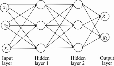
Fig. 1 Schematic of feed-forward neural network
3.2 Radial basis function neural network
RBFNN is obtained by introducing a number of modifications to the exact interpolation by the radial basis function [24, 25]. A RBFNN consists of three layers (as shown in Fig. 2) with the input layer consisting of N inputs, the hidden layers having m nodes and the output layer. Each of the nodes in the hidden layers receives multiple inputs from every input.
According to BISHOP [26] and HAYKIN [27],standard RBFNN interpolation for a training data set of (xi, g(xi)) can be represented as
 (8)
(8)
where wi and fi are weights and radial basis functions, respectively. There are many types of radial basis functions, but the most commonly used radial basis function is Gaussians. Hence the Gaussians radial basis function is used in this work, i.e.,
 (9)
(9)
where ai>0 is the width parameter and si is the center. The radial basis functions of x at each sampling points are determined by the above equation. Note that
 (10)
(10)
where ��i is the standard deviation of the Gaussians. In general, ��i is chosen as the minimum or average of the {(xi�Cxi�C1), (xi+1�Cxi)} so that if the node are equi-spaced, ai is the same for each radial basis function. There are two stages for training a RBFNN. In the first stage, the input data set is used to determine the parameters of the radial basis functions such as si and ��i. In the second stage, the parameters of the radial basis function are kept fixed and the second-layer weights are found. The second-layer weights are optimized by minimizing the error of approximated function performing iterative training of the network.
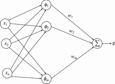
Fig. 2 Schematic of Radial basis function neural network
4 Procedure of presented method
Basic steps of performing structural reliability analysis using the combination of HDMR, ANN and MCS is as follows:
Step 1: The n sampling points are generated for each input variables along the variable axis xi. The response quantities at all sampling points of each input variable including reference point are calculated from the limit state function. Therefore, N sets of input and output are obtained for the training stage.
Step 2: Each sets of input-output are used to interpolate each of the low dimensional HDMR expansion terms with respect to the input values of the point x using ANN interpolation technique.
Step 3: Sum the interpolated values of HDMR terms from the zeroth order to the highest order of all the input variables. Here is an example for using the radial basis function
 (11)
(11)
Step 4: After training the ANN surrogate, the ANN surrogate is used to obtain the outputs of Ns random samples. The failure probability can be calculated as follows:
 (12)
(12)
where is the simulated output of x from the ANN surrogate, Ns is the sampling size, ��[��] is an indicator function of fail or safe state such that ��=1 if  otherwise zero.
5 Numerical examples
Three numerical examples are performed in this work to show the efficiency and accuracy of the presented method. These three numerical examples were already studied by previous researchers [4, 13, 28]. CHOWDHARY et al [13] used moving least square (MLS) method for the approximation of the limit state function. In this work, the MLP network and RBFNN are used for this purpose and the computational results are compared with those obtained by MCS to check the accuracy and efficiency of the presented techniques for HDMR. The coefficient of variance (COV), ��, of the estimated probability of failure PF using MCS for the sampling size Ns is computed as
 (13)
(13)
If COV is small then probability of failure computed by direct MCS can be regarded as the true value. Hence, this true value can be used to compare the accuracy of probability of failure obtained after HDMR-ANN approximation. Further, the percentage error is calculated at different sets of input variables. The percentage error can be mathematically expressed as
 (14)
(14)
The first order HDMR leads to explicit representations of implicit limit state functions. Therefore, MCS can be conducted with a small computational effort. The total number of function evaluations of the presented methods reduce to (n�C1)��N+1 [19]. The method of HDMR combined with MLP is abbreviated as HDMR-MLP and the method of HDMR combined with RBFNN is abbreviated as HDMR-RBFNN.
5.1 Example 1
An explicitly non-linear limit state function is selected as the first numerical example [28]. This limit state function was also studied by CHOWDHURY et al [13] by using HDMR. But they used MLS method for the interpolation. In this study, we adopted ANN instead of MLS method. The limit state function is given by
 (15)
(15)
where x1 and x2 are assumed to be independent random variables and have standard normal distribution with zero mean and unit standard deviation. This limit state function was approximated using HDMR and two types of ANN with number of epoch as 1000. Performance goal is to minimize the training error with a minimum gradient as 1��10�C7. The percentage error of true values and approximated component function values at five testing points are shown in Table 1. They are used to show the accuracy of the presented method. The probability of failure obtained using HDMR-MLP is 0.009124 (Table 2). The performance curves in Fig. 3 show that the mean squared error (MSE) are approaching towards the performance goals. The regression curves (Fig. 4) show the linear relationship between the original function values (target) and approximated function values (output). The line g=T, where g is output and T is target, means that the ANN surrogate is well fitted as all of the data fall along this line. Similarly, HDMR- RBFNN was also used to estimate the probability of failure. The probability of failure obtained using this method was 0.009335 which is closer to the Pf obtained by direct MCS (Table 2). The COV of PF (direct MCS) corresponding to 106 sampling size is 0.0102. Compared with direct MCS (Pf=0.0095), HDMR-MLP underestimates the failure probability by 3.95% (Pf= 0.009335) whereas HDMR-RBFN underestimates the failure probability by 1.736% (Pf=0.009335) (Table 2). The number of sampling points for each component function was 5, i.e., n=5. Therefore, the total number of function evaluation was nine, which is very small compared to the one million function evaluations by direct MCS.
Most of sampling points should fall along a 45��line (Fig. 4), where the network output is equal to the target.
Table 1 Percentage error at five testing points for example 1

Table 2 Failure probabilities obtained by different methods for example 1
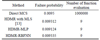
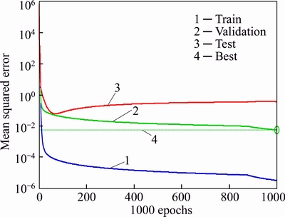
Fig. 3 Performance curves of HDMR-MLP for example 1
The R values in the regression plots should also be more than 0.90 for better fitting. As we can see in Fig. 4, most of sampling points are on 45�� line and the R values in the regression plots are very close to 1. Hence, this ANN surrogate is trained well. The stopping parameters of the training also determine the accuracy of the trained ANN surrogate. If the training process stops due to the reaching of minimum performance goal, then the trained ANN can be regarded as a better one, otherwise the network maybe need to be trained again. If the training process stops due to the reaching of the maximum number of epoch or validation then this may lead to an inaccurate ANN surrogate. Another strategy to avoid this consequence, the number of sampling points used may be increased which can lead to a more accurate ANN surrogate.
5.2 Example 2
This example was previously studied by PENMETSA and GRANDHI [4]. Burst margin is the margin of safety before an overstress condition occurs due to the stress on the part being too large for the material to withstand (Fig. 5). It is defined as the function of the material utilization factor (am), the ultimate tensile strength (Su), density (��), rotor speed (��) and outer (Ro) and inner (Ri) radii of the disk. The ultimate tensile strength is the maximum stress and the material utilization factor is the safety factor accounting for uncertainties and unknown material properties. The density of the material, the disk speed, and the thickness of the disk are used to determine the average tangential stress
 (16)
(16)
The satisfactory performance of the disk is defined when the burst margin, Mb, exceeds the threshold value of 0.37473 [4]. Therefore, the limit state function is defined as
 (17)
(17)
Statistical properties of input random variables are given in Table 3.
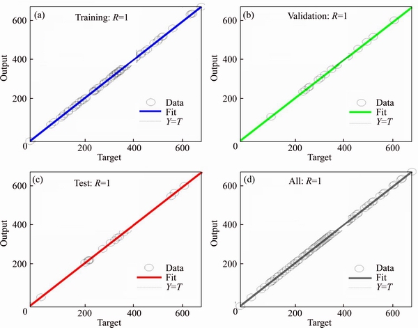
Fig. 4 Regression plots of HDMR-MLP for example 1
The number of sampling points for approximating the first order HDMR component function is 5, i.e., n=5. Therefore, the total number of function evaluations is 25, while one million function evaluations are used by direct MCS. The percentage errors of true values and approximated function values at five testing points are shown in Table 4. The results of the presented method are compared with MCS in order to check the accuracy and efficiency of this presented method (Table 5). The probability of failure obtained by direct MCS is 0.00101. The COV of Pf (MCS) corresponding to 106 sampling size is 0.0314. Compared with MCS (Pf=0.00101),HDMR-MLP (Pf=0.0029) overestimates the failure probability by 187.9% whereas HDMR-RBFNN (Pf=0.0018) overestimate the failure probability by 78.21%. However, the magnitude of these two estimators is in the same order of the true values, which meets the engineering requirements. Figure 6 shows the performance curves for the current problem, and Fig. 7 gives the associated regression curves. Similar conclusions to example 1 can be drawn from these two figures.
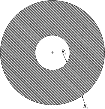
Fig. 5 Rotating disk
Table 3 Statistical properties of input random variables

Table 4 Percentage error at five testing points for example 2
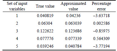
Table 5 Failure probabilities by different methods for example 2
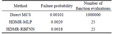

Fig. 6 Performance curves of HDMR-MLP for example 2
5.3 Example 3
This example was previously studied by PENMETSA and GRANDHI [4]. A ten-bar truss structure, as shown in Fig. 8, is considered to examine the accuracy and efficiency of this presented method. The elastic modulus of material is 6.895��107 kPa. Two concentrated forces of 105lb are applied at nodes 2 and 4, as shown in the Fig. 8. The cross-sectional areas of the bars are considered as normal random variables with mean of 2.5 in2 and standard deviation of 0.5 in2. According to the loading condition, the maximum displacement u2(x1, x2, ��, x10) occurs at node 2, where a permissible displacement is limited to umax=18in. Hence the limit state function of this structure is defined as
 (18)
(18)
Both HDMR-MLP and HDMR-RBFNN are applied to evaluate the failure probability of the structure.Table 6 shows the percentage errors at five testing points, and Table 7 gives the results obtained by MCS and the proposed methods. The COV of Pf (MCS) corresponding to 106 sampling size is 0.002484. Compared with the direct MCS (Pf=0.1394), HDMR-MLP (Pf=0.19) overestimate the failure probability by 36.3%, whereas HDMR-RBFNN (Pf=0.1356) under estimates the failure probability by �C2.72%. The number of sampling points for approximating each component function was 5, i.e., n=5. Therefore, the total number of function evaluation was 41, while one million function evaluations is still used by direct MCS. The percentage error of true values and approximated function values at five testing points are shown in Table 6. Figure 9 shows the performance curves for the current problem, and Fig. 10 gives the associated regression curves. Similar conclusions to examples 1 and 2 can be drawn from these two figures.
6 Conclusions
The limit state functions are usually implicitly defined through numerical models for the structural analysis of the real life problems. This paper presented a new computational method for estimating the probability of failure of structures. It utilizes the excellent properties of HDMR for multivariate function approximation and ANN as the interpolation scheme. Two different types of ANN are adopted to approximate the original limit state function. HDMR combined with ANNs can approximate the limit state function with better accuracy and less computational efforts. The surrogate model using HDMR and ANN can be used to obtain the structural responses for any random samples. But while training an ANN surrogate, attention should be paid on regarding the occurrence of data on the regression plots. Three numerical examples are used to illustrate the performance of this method. Comparisons are made with direct MCS. The computational results show that the presented method not only yields the accurate results but also reduces its computational efforts compared to direct MCS. The probabilities of failure obtained by HDMR- RBFNN are more close to those obtained by direct MCS than HDMR-MLP.

Fig. 7 Regression plots HDMR-MLP for example 2

Fig. 8 Bar truss structure
Table 6 Percentage error at five testing points for example 3
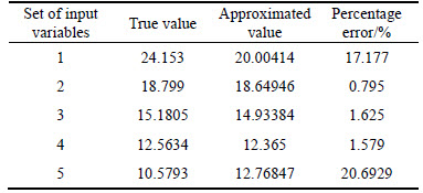
Table 7 Failure probabilities by different methods for example 3
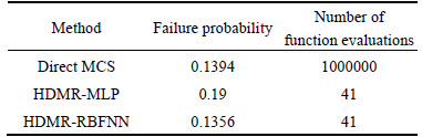

Fig. 9 Performance curves of HDMR-MLP for example 3
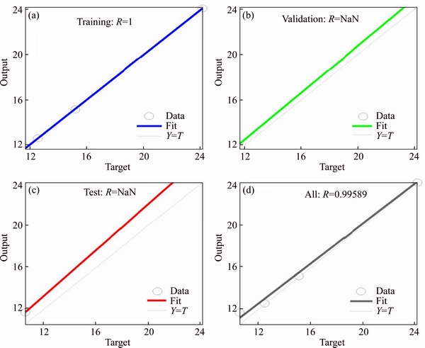
Fig. 10 Regression plots of HDMR-MLP for example 3
References
[1] DITLEVSEN O, MADSEN H O. Structural reliability methods [M]. Chichester: John Wiley & Sons, 1996.
[2] BUCHER C. Computational analysis of randomness in structural mechanics [M]. London: CRC Press, 2009.
[3] LIU P L, DERKIUREGHIAN A. Finite element reliability of geometrically nonlinear uncertain structures [J]. Journal of Engineering Mechanics, 1988, 117(8): 164�C168.
[4] PENMETSA R C, GRANDHI R V. Adaptation of fast Fourier transformations to estimate structural failure probability [J]. Finite Elements in Analysis and Design, 2003, 39(5, 6): 473�C485.
[5] WU Y T, TORNG T R. A fast convolution procedure for probabilistic engineering analysis [C]// Proceeding of the First International Symposium on Uncertainty Modeling and Analysis. College park, Maryland, USA: IEEE, 1990: 670�C675.
[6] ZHAO Y G, ONO T. Moment methods for structural reliability [J]. Structural Safety, 2001, 23(1): 47�C75.
[7] LU Z H, ZHAO Y G, ANG A H S. Estimation of load and resistance factors based on the fourth moment method [J]. Structural Engineering and Mechanics, 2010, 36(1): 19�C36.
[8] ZHAO Y G, LU Z H. Applicable range of the fourth-moment method for structural reliability [J]. Journal of Asian Architecture & Building Engineering, 2007, 6(1): 151�C158.
[9] RUBINSTEIN R Y, KROSES D P. Simulation and the Monte Carlo method [M]. New Jersey: John Wiley & Sons, 2017.
[10] SOBOL I M. Theorems and examples on high dimensional model representations [J]. Reliability Engineering and System Safety, 2003, 79(2): 187�C193.
[11] SOBOL I M. Sensitivity analysis for non-linear mathematical models [J]. Mathematical Modeling & Computational Experiment, 1993, 1(4): 407�C414.
[12] RAO B N, CHOWDHURY R. Probabilistic analysis using high dimensional model and fast Fourier transform [J]. International Journal for Computational Methods in Engineering Science and Mechanics, 2008, 9(6): 342�C357.
[13] CHOWDHARY R, RAO B N, PRASAD A M. High dimensional model representation for structural reliability analysis [J]. Communications in Numerical Methods in Engineering, 2009, 25(4): 301�C337.
[14] RAO B N, CHOWDHARY R, SINGH C R, KUSHWAHA H S. Structural reliability analysis of AHWR and PHWR inner containment using high dimensional model representation [C]// Proceedings of 2nd International Conference on Reliability, Safety & Hazard (ICRESH-2010). Mumbai, India: IEEE, 2010: 78�C86.
[15] WANG H, TANG L, LI G Y. Adaptive MLS-HDMR metamodeling techniques for high dimensional problems [J]. Expert Systems with Applications, 2011, 38(11): 14117�C14126.
[16] SHAN S, WANG Gary. Development of adaptive RBF-HDMR model for approximating high dimensional problems [C]// Proceedings of the ASME 2009 International Design Engineering Technical Conferences & Computers and Information in Engineering Conference. San Diego, California, USA: ASME, 2009: 727�C740.
[17] ZHOU C C, LU Z Z, LI G J. A new algorithm for variance based importance measures and importance kernel sensitivity [J]. Proceedings of the Institution of Mechanical Engineers Part O: Journal of Risk and Reliability, 2013, 227(1): 16�C27.
[18] LI G, ROSENTHAL C, RABITZ H. High dimensional model representation [J]. Journal of Physical Chemistry, 2001, 105(55): 7765�C7777.
[19] RABITZ H, ALIS O F. General foundations of high-dimensional model representations [J]. Journal of Mathematical Chemistry, 1999, 25(2, 3): 197�C233.
[20] CHOWDHURY R, RAO B N, PRASAD A M. High dimensional model representation for piece wise continuous function approximation [J]. Communications in Numerical Methods in Engineering, 2008, 24(12): 1587�C1609.
[21] MACLEOD C. An introduction to practical neural networks and genetic algorithms for engineers and scientists [M]. Scotland: The Robert Gordon University, 2010.
[22] LEVENBERG K. A method for the solution of certain non-linear problems in least squares [J]. Quarterly of Applied Mathematics, 1944, 2(2): 164�C168.
[23] MARQUARDT D W. An algorithm for least square estimation for non-linear parameters [J]. Journal of the Society for Industrial and Applied Mathematics, 1963, 11(2): 431�C441.
[24] BROOMHEAD D S, LOWE D. Multivariable functional interpolation and adaptive networks [J]. Complex Systems, 1988, 2(1): 321�C355.
[25] MOODY J, DARKEN C J. Fast learning in networks of locally tuned processing units [J]. 1989, 1(2): 281�C294.
[26] BISHOP CM. Neural networks for pattern recognition [M]. Oxford: Clarendon Press, 1995.
[27] HAYKIN S. Neural Networks: A comprehensive foundation [M]. New Jersey: Prentice-Hall, 1999.
[28] KIM S H, NA S W. Response surface method using vector projected sampling points [J]. Structural Safety, 1997, 19(1): 3�C19.
(Edited by HE Yun-bin)
Cite this article as:
Bhaw Nath Jha, LI Hong-shuang. Structural reliability analysis using a hybrid HDMR-ANN method [J]. Journal of Central South University, 2017, 24(11): 2532�C2541.
DOI:https://dx.doi.org/https://doi.org/10.1007/s11771-017-3666-7Foundation item: Project(U1533109) supported by the National Natural Science Foundation, China; Project supported by the Priority Academic Program Development of Jiangsu Higher Education Institutions, China
Received date: 2015-12-14; Accepted date: 2016-08-01
Corresponding author: LI Hong-shuang, PhD, Associate Professor; Tel: +86�C25�C84890119; Fax: +86�C25�C84891422; E-mail: hongshuangli@nuaa.edu.cn
Abstract: A new hybrid method is proposed to estimate the failure probability of a structure subject to random parameters. The high dimensional model representation (HDMR) combined with artificial neural network (ANN) is used to approximate implicit limit state functions in structural reliability analysis. HDMR facilitates the lower dimensional approximation of the original limit states function. For evaluating the failure probability, a first-order HDMR approximation is constructed by deploying sampling points along each random variable axis and hence obtaining the structural responses. To reduce the computational effort of the evaluation of limit state function, an ANN surrogate is trained based on the sampling points from HDMR. The component of the approximated function in HDMR can be regarded as the input of the ANN and the response of limit state function can be regarded as the target for training an ANN surrogate. This trained ANN surrogate is used to obtain structural outputs instead of directly calling the numerical model of a structure. After generating the ANN surrogate, Monte Carlo simulation (MCS) is performed to obtain the failure probability, based on the trained ANN surrogate. Three numerical examples are used to illustrate the accuracy and efficiency of the proposed method.
