
J. Cent. South Univ. (2016) 23: 189-200
DOI: 10.1007/s11771-016-3062-8

Theoretical generalization of Markov chain random field from potential function perspective
HUANG Xiang(����)1, WANG Zhi-zhong(��־��)1, GUO Jian-hua(������)2
1. School of Mathematics and Statistics, Central South University, Changsha 410083, China;
2. School of Geosciences and Info-Physics, Central South University, Changsha 410083, China
 Central South University Press and Springer-Verlag Berlin Heidelberg 2016
Abstract:
The inner relationship between Markov random field (MRF) and Markov chain random field (MCRF) is discussed. MCRF is a special MRF for dealing with high-order interactions of sparse data. It consists of a single spatial Markov chain (SMC) that can move in the whole space. Generally, the theoretical backbone of MCRF is conditional independence assumption, which is a way around the problem of knowing joint probabilities of multi-points. This so-called Naive Bayes assumption should not be taken lightly and should be checked whenever possible because it is mathematically difficult to prove. Rather than trap in this independence proving, an appropriate potential function in MRF theory is chosen instead. The MCRF formulas are well deduced and the joint probability of MRF is presented by localization approach, so that the complicated parameter estimation algorithm and iteration process can be avoided. The MCRF model is then applied to the lithofacies identification of a region and compared with triplex Markov chain (TMC) simulation. Analyses show that the MCRF model will not cause underestimation problem and can better reflect the geological sedimentation process.
Key words:
localization approach; Markov model; potential function; reservoir simulation; transiogram fitting��
1 Introduction
Markov chain (MC) model was introduced by Markov in 1906 and applied to stratigraphy by VISTELIUS [1]. One-dimensional (1-D) Markov chains (or transition probabilities) have long been used in geosciences [2�C3]. Multi-dimensional (M-D) Markov chain models can be traced to KRUMBEIN [4] and LIN and HARBAUGH [5] in geology for modeling lithological (or sedimentological) structures. The M-D Markov chain model proposed by ELFEKI and DEKKING [6] considered the nearest known neighbors in cardinal directions with the fully independent assumption. M-D Markov chain is composed of fully independent 1-D Markov chains and these chains are forced to move to equal states [6]. The fully independent assumption caused directional effect (i.e., pattern inclination or diagonal trend) and the small-class underestimation problem. It has been found that the exclusion of unwanted transitions causes lower values of small class proportion or higher values of large class proportion. The directional effect problem was actually a long-standing problem in unconditional M-D Markov chain simulations for image texture analyses, which was caused by asymmetric neighborhoods used in simulations [7].
Markov chains are usual tools, which can be helpful to describe temporal sequences of random variables, governed by transition probabilities; the system ��state�� in the series is represented by the value of the random variable. Markov random field (MRF) is defined as an extension of the Markov chains, where the random variable is replaced by the random function, and the system ��state�� is the spatial image of the variable. SALOM O and REMACRE [8] discussed relevant aspects concerning the use of discrete MRF in the simulation of rock properties in petroleum reservoirs, and they use Metropolis algorithm to compute the calculus of the practical semi-variogram function in the binary Markov images. NORBERG et al [9] extended the locally based prediction methodology of Bayesian- Markov to a global one by modeling discrete spatial structures as Markov random fields. It provides an important development compared to the Bayesian- Markov methodology by facilitating global predictions and improves use of sparse data, while more work is needed in order to simulate, since it appears to have a tendency to overestimate strong spatial dependence.LIU et al [10] discussed the principle of simulating continuous reservoir attributes based on Gaussian MRF. LIANG et al [11] used MRF tool to simulate lithofacies distribution and proposed a Gibbs distribution to characterize reservoir heterogeneity.
All these works are done by either MC or MRF, but few have found the inner relationship between the two. In fact, Markov chain random field (MCRF) is the perfect answer. LI [12] proposed this and solved the small-class underestimation problem, which has long existed in M-D Markov chain simulation. The MCRF theory defines a single spatial Markov chain (SMC) that moves in an M-D space, with its transition probabilities at each given location entirely depending on its nearest neighbors in different directions under the conditional independence assumption [12�C13]. In an MCRF, it is assumed that there is only one single Markov chain in a space which has its conditional probability distribution (CPD) at any location entirely dependent on its nearest ��known�� neighbors in different directions. An MCRF should be a special MRF because it obeys the transition probability law. The difference is that the former is built on a ��directional chain�� and the latter does not contain chains.
The MCRF concept, a new idea for geostatistics or a primitive theory for spatial modeling purposes, was not sufficiently described mathematically in previous publications [14]. We need rigorous treatment to the MCRF idea. The problem is discussed and solved on the basis of Markov random field theory in this work. We choose the canonical potential function in MRF to deduce the MCRF formulas.
2 Markov chain model
A Markov chain is a probabilistic model that exhibits a special type of dependence: given the present, the future does not depend on the past. In formulas, let Z0, Z1, Z2, ��, Zm be a sequence of random variables taking values in the state space {S1, S2, ��, Sn}. The sequence is a Markov chain or Markov process if

 (1)
(1)
where ��|�� is the symbol for conditional probability, and �� �� is for notation convenience.
The coupled Markov chain (CMC) proposed by ELFEKI and DEKKING [6] describes the joint behavior of a pair of independent systems, each evolving according to the laws of a classical Markov chain [15]. Consider two Markov chains, (Xi) and (Yj), both defined on the state space {S1, S2, ��, Sn} and having the positive transition probability defined as
 (2)
(2)
The coupled transition probability plm,kf on the state space {S1, S2, ��, Sn}��{S1, S2, ��, Sn} is given by
 (3)
(3)
Two-coupled one-dimensional Markov chains, (Xi) and (Yj), can be used to construct a two-dimensional spatial stochastic process on a lattice (Zi,j). The stochastic process (Zij) is obtained by coupling the (Xi) and (Yj) chain, but forcing these chains to move to equal states. Hence,

 (4)
(4)
where C is a normalizing constant that arises by not permitting transitions in the (Xi) and (Yj) chain to different states.
The triplex Markov chain (TMC) methodology discussed in Ref. [16] uses two CMCs constructed from three independent one-dimensional first-order Markov chains. Consider three one-dimensional stationary Markov chains  and (Yj) all defined on the state space {S1, S2, ��, Sn}. The symbol (Yj) represents a y direction chain. The
  and
and  represent an x direction chain (i.e., from left to right) and an �Cx direction (i.e., anti-x-direction, from right to left) chain, respectively. Then, the (Yj) andare coupled together to form one CMC
 from left to right, and at the same time (Yj) and are coupled together for the other CMC
  from right to left. The two CMCs proceed on a two-dimensional domain at opposite directions alternately.
LIANG et al [11] proposed the triplex Markov chain (TMC) in 3-D space. The conditional probability distribution of 3-D TMC at any unknown location can be written as

 (5)
(5)
where represent transition probabilities in coordinate directions.
Both the CMC model and the TMC model use couplings of multiple 1-D Markov chains. This means they are multiple-chain models. The occurrence of the small-class underestimation problem is exactly related to the use of multiple chains.
3 Localized MRF approach
MRF is defined as an extension of the Markov chains. Let F be a random field on site set S with respect to the neighborhood system ��, and F=(F1, F2, ��, Fn) is said to be a MRF if and only if the positivity Eq. (6) and the Markovianity Eq. (7) are satisfied:

 (6)
(6)
 (7)
(7)
where S�C{s} is the set difference, fS�C{s} denotes the set of labels at the sites in S�C{s} and  stands for the set of labels at the sites neighboring s:
 (8)
(8)
The positivity is assumed for some technical reasons and can usually be satisfied in practice. For example, when the positivity condition is satisfied, the joint probability P(f ) of any random field is uniquely determined by its local conditional probabilities [17]. The Markovianity depicts the local characteristics of F. In MRFs, only neighboring labels have direct interactions with each other. If we choose the largest neighborhood in which the neighbors of any sites include all other sites, then any F is an MRF with respect to such a neighborhood system [18].
The joint probability P(f) of an MRF takes the following form:
 (9)
(9)
It obeys a Gibbs distribution according to the Hammersley-Clifford theorem [19], where T is a constant called the temperature which is assumed to be 1. The energy U(f) is a sum of clique potentials Vc(f) over all possible cliques C:is the partition function. Figure 1 illustrates the neighborhood defined by causal MRF model in an M-D space, where the cliques are the current positions connected with adjacent sites with one edge, two edges, three edges and so on. Cliques with n edges are denoted by C1, C2, ��, Cn. Note that MRF is traditionally defined as undirected graph in graph theory.


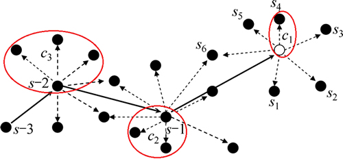
Fig. 1 Neighborhood defined by a causal MRF model in an M-D space (Cliques are current positions connected with adjacent sites with one edge c1, two edges c2, three edges c3 and so on; White cell refers to current location with an unknown state, and surrounding black cells represent its nearest known neighbors in different directions in simulation domain (or in a search radius); Arrows represent energy transfer direction)
The arrows in Fig. 1 represent energy transfer direction.
It is known that the choices of clique potential functions for a specific MRF are not unique; there may exist many equivalent choices which specify the same Gibbs distribution. However, there exists a unique normalized potential, called the canonical potential, for every MRF [20]. The canonical potential function is defined by

where f denotes the empty set, |c�Cb| is the number of elements in the set c�Cb and is the configuration which agrees with f on set b but assigns the value 0 to all sites outside of b:

For nonempty c, the potential can also be obtained as
 (10)
(10)
where i is any element in b.
 can be rewritten as

We first consider site s with three neighbors s1, s2 and s3. The potential function Vn can be denoted by


Thus, the energy function with three neighbors in an MRF is


 (11)
(11)
The above equation implies a homogeneous Gibbs distribution because V1, V2 and V3 are independent of the locations si, s1, s2 and  For non-homogeneous Gibbs distribution, the cliques function should be written as
  and
and  and so on. In general, the expression of Vn is

 (12)
(12)
In this way, the general expression of energy function with n neighbors in an MRF can be derived as

 (13)
(13)
where n��3 and n is an odd number. Substituting Eq. (10) into Eq. (9), the joint probability of an MRF can be denoted as

 (14)
(14)
Hence, the joint probability of an MRF can be expressed by the product of local conditional probabilities. The complicated parameter estimation algorithm and iteration process can be avoided by computing local conditional probabilities. So, the highly time-consuming problem of MRF mentioned in Ref. [21] has been solved.
4 Relationship between MRF and MCRF
Let F be an MRF on S with respect to the neighborhood system ��, A is a set consisting of cliques containing i, and the conditional probability depends only on the potentials of the cliques in set A:
 (15)
(15)
That is to say, it depends on labels at i��s neighbors. Its proof can be found in Ref. [18]. According to MRF��s local property, we also have
 (16)
(16)
We can obtain the M-D Markov chains from Eq. (10) by considering cliques c1 with only one edge in the MRF, for the sake of finding the connection between MRF and MCRF [22].
Noting that edge in the clique has a direction property, the energy function can be denoted as


 (17)
(17)
Put c=2 and b=1 in Eq. (10). Substituting Eq. (17) into Eq. (15), we obtain


 (18)
(18)
We obtain

 (19)
(19)
If we use transition probabilities with distance lags to replace two-point conditional probabilities in Eq. (18), there is

 (20)
(20)
where C is a constant,  represents a transition probability in the ith direction from state fs to state
  with a lag hi;
  represents a transition probability in the moving direction (energy transfer direction) from previous state fs�C1 to current state fs with a lag h. With increasing lag h, any forms a transition probability diagram, which is called ��transiogram�� in MCRF theory. Renormalizing the right hand side of Eq. (20) to cancel the constant C, there is


 (21a)
(21a)
LI [12] proposed the general expression of the SMC X in an MCRF theory based on conditional independence assumption, which is given as

 (21b)
(21b)
The conditional independence assumption is hard to satisfy in real geological unit, and we turn to study the potential function in MRF theory. Equation (21a) gives the general expression of the local conditional probability in an MRF, which is fully in accordance with the local conditional distribution (CPD) of the SMC Eq. (21b) at any unknown location in an MCRF. The exact form of Eq. (21) at a specific location depends on the number of the nearest known neighbors found in different directions, distances from these nearest known neighbors to the location to be estimated, and directions along which the energy transfers. From Eq. (14) and Eq. (21), the joint probability of an MRF is derived as
 (22)
(22)
An SMC model Eq. (21b) in an MCRF and an MRF Eq. (7) are all defined on their neighbor sets and are all generalizations of a Markov chain in multiple dimension. Therefore, MCRF is a special MRF with a single ��directional chain�� [23�C24].
5 Transiogram model
Transiogram [25] plays a very important role in MCRF simulation. To obtain continuous transiogram models from discontinuous experimental transiograms (which are directly estimated from sample data), one may construct mathematical models to fit experimental transiograms [26] or just interpolate experimental transiograms into continuous models [27]. In addition, for exclusive classes, the nugget effect is irrational to transition probabilities and should not be considered in transiogram modeling [24]. Transiograms can be directly estimated from sampled data by counting the transition frequencies of classes with different lags (numbers of pixels for raster data), just like estimating a one-step transition probability matrix, which has only one fixed lag of h=1 in a discrete space [28]. The equation is given as
 (23)
(23)
where Tlk(h) is the transition probability with lag h.
The vertical transition probabilities can be easily computed by the well data in the work area. The transition probabilities from lithofacies l to k is defined as

where Tlk is the transition tally from lithofacies l to k. When the outcrop data are absent, the horizontal transition probabilities can be acquired from the vertical transition probabilities by using Walther��s Law, where vertical successions represent the lateral succession of environments of deposition [29�C30]. Suppose that the vertical transition tally of the stratum is Nz, and the apparent dips in vertical section from west to east and south to north are �� and ��, respectively. Therefore, the transition tally matrices from west to east and south to north in horizontal direction are Nx and Ny, respectively. The transition tally matrices are shown as
 (24)
(24)
 (25)
(25)
 (26)
(26)
where nij represents the transition tally from lithofacies i to j; ni is the frequency of lithofacies i with thickness greater than step size; lz, lx and ly represent the step sizes in vertically downward, west to east, south to north direction, respectively. For more detail, see Ref. [31].
The transiogram can be obtained by plk with different lag h. Some experimental transiograms have apparent fluctuations that are difficult to fit using the basic model, such as exponential model or spherical model. Fitted transiogram models capture only part of the features of experimental transiogams, depending on the complexity of the mathematical models used [13]. Using composite hole-effect models [32] for composite hole-effect models for auto-variograms may capture more details, such as periodicities, of experimental transiogams.
The dampened hole-effect model [33], that is, the multiplicative cosine-exponential composite model, can be directly used as a transiogram model to fit experimental cross-transiograms with similar hole-effect features [34�C36]. As a cross-transiogram model, the multiplicative cosine-exponential composite model is given as
 (27)
(27)
where h is the lag distance, e is the sill, d is the effective range, and a is the wavelength of the cosine function. Since the hole effect, that is, the alternate peaks and troughs appearing on real experimental variograms or transiograms, is rarely regular, it is actually difficult to fit a series of peaks and troughs [37]. Considering that the useful part of a transiogram model for simulation is just the low lag section, we aim to fit only the first peak and trough of experimental cross-transiograms using this composite model.
6 Case study
6.1 Data sets
The data we used for our research are gathered from Tahe area of the Tarim Basin in Xinjiang Uygur Autonomous Region, China. There are three major lithologic facies in this area: mudstone, sandstone and conglomerate. The conglomerate is relatively low in content. We have got four wells�� lithologic data in the three-dimensional space (Fig. 2).
Three wells are located in the corners of this work area, and another well is located inside. The distance in east-west direction of the two wells is 6000 m, and 8000 m in south-north direction. The simulated space is split into a 60��80��100 grid system, with each cell being a 100 m��100 m��1 m cuboid. According to the geological drilling results, the average apparent dips in vertical section from west to east and south to north are 0.09�� and 0.11��, respectively.
6.2 Estimated transiogram
The transition tally matrices in vertical direction and horizontal direction are shown in Fig. 3. Experimental unidirectional transiograms were estimated from the dataset with 1765 samples from the drilling system. The measured transition probabilities were then fitted by cosine-exponential composite model. The fitted transiogram models were used for simulations. Because raster data were used, the lag h was represented as the number of pixels (i.e., grid units), not the exact distance.
Figures 4 and 5 illustrate the experimental auto/ cross transiograms and their fitting models in vertical direction and horizontal direction, respectively. From the start point (0,1), we may draw a tangent of the auto-transiogram to the x�Caxis. The lag h where the tangent crosses the x-axis is equal to the mean vertical thickness or horizontal extension length [38]. For example, sandstone mean vertical thickness is 2 m (Fig. 4(a)). Transiogram p12(h) (Fig. 5(b)) and p21(h) (Fig. 5(d)) both have a peak first and then approach its sill, which means Class 1 (sandstone) frequently occurs adjacent to Class 2 (mudstone). Transiogram p13(h) and p31(h) always have a low-value section first and then approach its sill (Fig. 4(c) and Fig. 4(g)), which means Class 1 (sandstone) seldom occurs close to Class 3 (conglomerate). In fact, conglomerate is more likely to appear where sandstone develops according to priori geological experience.
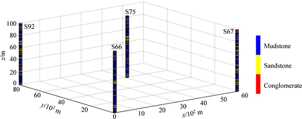
Fig. 2 3-D work area with 4 wells (S66, S67, S75 and S92)
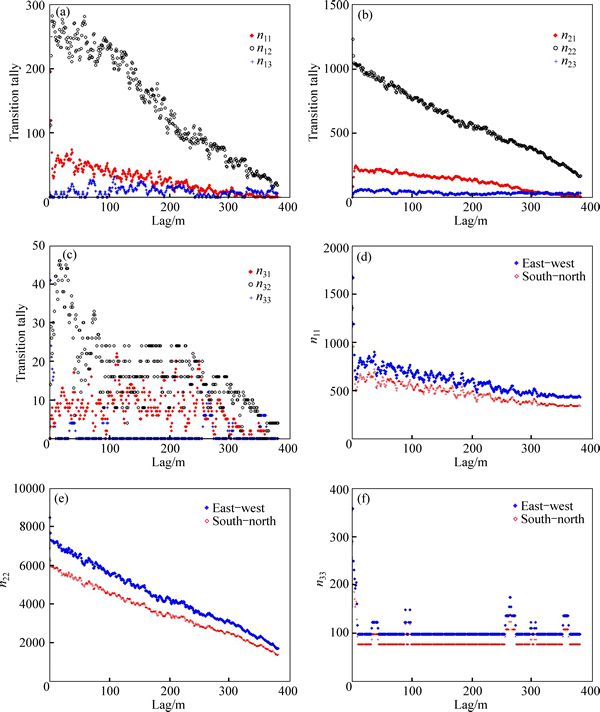
Fig. 3 Transition tally matrices in vertical direction (a, b and c) and horizontal direction (d, e and f)
It can be seen that most of these experimental transiograms can be approximately fitted by cosine- exponential models. We also find that some experimental transiograms have apparent fluctuations that are difficult to fit using the basic model, such as p13 and p33. This may be caused by the insufficiency of observed data and the non-Markovian effect of the real data.
6.3 Simulated results and analysis
According to the four wells and step size we choose, the unknown grid in this work area is simulated by using MCRF algorithm. In this 3-D space, only considering cardinal directions, we can get a general 3-D SMC model as

 (28)
(28)
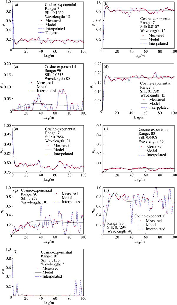
Fig. 4 Unidirectional experimental transiograms estimated from well data along vertical direction
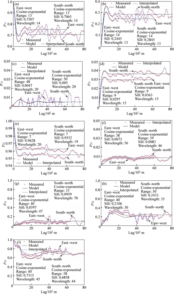
Fig. 5 Unidirectional experimental transiograms along horizontal direction
Thus, we have six conditional points in the searching neighborhood. The four realizations of lithologic stochastic simulation are shown in Fig. 6. The four realizations generally reflect the basic rule of sand body development in this area. The sandstone thickness is mostly 1�C5 m, presenting a thin layer of output. It is continuous in horizontal direction, which can extend to several kilometers. Mudstone is the background lithofacies, and widely distributes in this area. Conglomerate is not well developed in this work area, which is not continuous neither in vertical direction nor in horizontal direction. On one hand, we can safely draw a conclusion from Fig. 6 that the conglomerate can onlyextend 200�C300 m in horizontal direction, and the average thickness of this type of lithofacies is no more than 3 m. The simulation result is in accordance with the transiogram mean length analysis. On the other hand, the conglomerate is more likely to appear in sandstone distribution area, which means that the transition probability between conglomerate and sandstone is higher than that of mudstone. Mudstone and sandstone are more continuous than conglomerate in horizontal direction, and the occurrence frequency of mudstone is significantly greater than the other lithofacies in vertical direction. This performance is in accordance with the transition probability function (transiogram) in each direction.
To clearly display spatial uncertainty, a practical way is to use occurrence probability maps estimated from a number of simulated realizations. The maximum occurrence probability map generated by a simulation demonstrates the spatial uncertainty associated with the optimal prediction map, which may be comparable with a delineated map based on the same sample data. Figure 7 shows the maximum occurrence probability maps of mudstone generated by MCRF, conditioned on 1765 samples from the drilling system and estimated from 100 realizations for each simulation. It can be seen that the occurrence probability of mudstone is relatively high in the gray image, which means that mudstone is widely spread as a background lithology. In some areas, the occurrence probability of mudstone is close to zero, which means that sandstone or conglomerate is developed here. The probability distribution has high credibility, as proven by the realizations of lithologic stochastic simulation (Fig. 6).
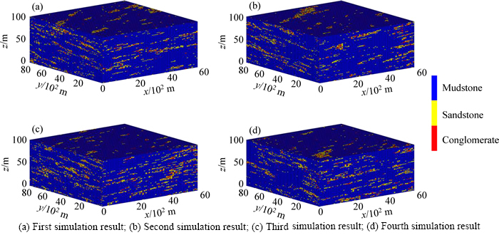
Fig. 6 Four realizations of MCRF lithofacies stochastic simulation:
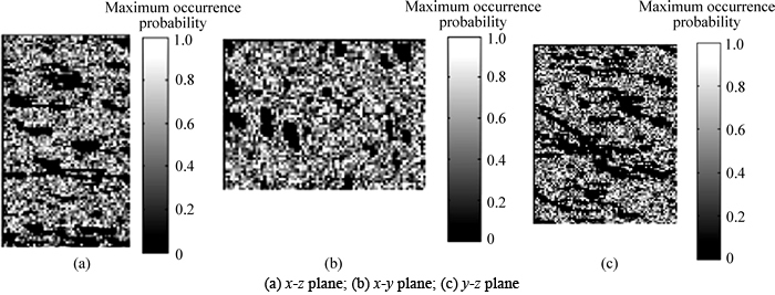
Fig. 7 Maximum occurrence probability maps of mudstone generated by MCRF algorithm, conditioned on 1765 samples from drilling system and estimated from 100 realizations for each simulation:
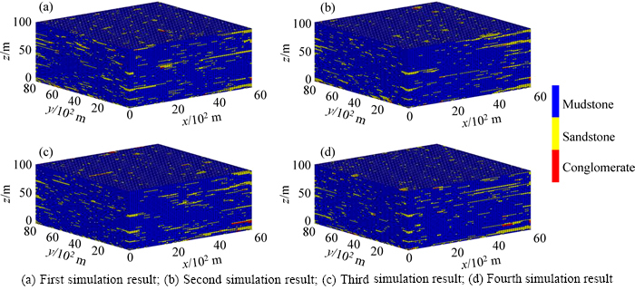
Fig. 8 Four realizations of TMC lithofacies stochastic simulation:
6.4 Comparison with TMC simulation
A procedure for Monte Carlo sampling to implement the TMC simulation methodology is as follows.
Step 1: Use proper sampling intervals in the three- dimensional work area.
Step 2: Transiograms are fitted in cardinal direction.
Step 3: Generate the rest states of the cells using the local conditional probability (LCP):

where the states at  are known. From state l1 at the x-axis neighboring cell (i�Cl, j, k), l2 at the y-axis neighboring cell (i, j�C1, k), and l3 at the vertical neighboring cell (i, j, k�C1), one can simulate the succeeding state l at cell (i, j, k) by Eq. (5).
Step 4: After having visited all cells in the domain, we obtain one realization.
Step 5: Repeat Step 3 and Step 4.
According to the simulation procedure, the simulated results are shown in Fig. 8. Compared with Fig. 6, the sandstone layer is thinner in vertical direction and conglomerate is rarer distributed, which means that this TMC method may underestimate the small class proportion. This conjecture is verified in Table 1.
Table 1 Lithofacies proportions in well data and averaged from four simulated realizations
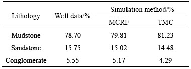
In our analysis, the well data (Table 1) are used for validation. We can safely conclude that, compared with TMC model, MCRF method is relatively better at maintaining the percentage composition of each lithofacies.
7 Conclusions
The focus of this work is the theoretical foundation of Markov chain random field (MCRF) and relationship between MRF and MCRF. However, a simple reservoir lithofacies simulation is also given to illustrate the availability of MCRF method. The transiogram fitting is not always perfectly satisfied due to the restriction of drilling system (we have only four wells�� data, and the conglomerate content is relatively low). MCRF algorithm has more advantage in coping with M-D simulation compared to MC method and better maintaining the geological attribute. Simulation result shows that the model is highly efficient in computation cost and well performed in handling sparse dateset situation. Yet neither MRF nor MCRF algorithm is available in most geological modeling software. Our simulation is implemented via MATLAB programming.
Acknowledgments
The authors thank Dr. CHEN Dong-dong for helpful discussion regarding the three-dimensional stochastic simulation and Dr. WU Kan for his valuable help on transiograms fitting.
References
[1] Vistelius A B.On the question of the mechanism of formation of strata [J]. Doklady Akademii Nauk SSSR, 1949, 65(2): 191�C194.
[2] Krumbein W C, Dacey M F. Markov chains and embedded Markov chains in geology [J]. Mathematical Geology, 1969, 1(1): 79�C96.
[3] Carle S F, Fogg G E. Modeling spatial variability with one and multi-dimensional continuous-lag Markov chains [J]. Mathematical Geology, 1997, 29(7): 891�C918.
[4] Krumbein W C. FORTRAN IV computer program for simulation of transgression and regression with continuous-time Markov models [D]. Evanston, Illinois: Northwestern University, 1968.
[5] Lin C, Harbaugh J W. Graphic display of two and three dimensional Markov computer models in geology [M]. New York: John Wiley & Sons, Inc, 1984: 180.
[6] Elfeki A, Dekking M A. A Markov chain model for subsurface characterization: Theory and applications [J]. Mathematical Geology, 2001, 33(5): 569�C589.
[7] Gray A J, Kay J W, TITTERINGTON D M. An empirical study of the simulation of various models used for images [J]. IEEE Transactions on Pattern Analysis and Machine Intelligence, 1994, 16(5): 507�C513.
[8] SALOMO M C, Remacre A Z. The use of discrete Markov random fields in reservoir characterization [J]. Journal of Petroleum Science and Engineering, 2001, 32(2): 257�C264.
[9]  , Baran S. On modelling discrete geological structures as Markov random fields [J]. Mathematical Geology, 2002, 34(1): 63�C77.
[10] Liu Zhen-feng, Hao Tian-yao, Wang Feng. Stochastic simulating distribution of continuous reservoir attributes based on the GMRF model [J]. Petroleum Exploration and Development, 2005, 32(6): 75�C81. (in Chinese)
[11] Liang Y, Wang Z, Guo J. Reservoir lithology stochastic simulation based on Markov random fields [J]. Journal of Central South University, 2014, 21(9): 3610�C3616.
[12] Li W. Markov chain random fields for estimation of categorical variables [J]. Mathematical Geology, 2007, 39(3): 321�C335.
[13] Li W. A fixed-path Markov chain algorithm for conditional simulation of discrete spatial variables [J]. Mathematical Geology, 2007, 39(2): 159�C176.
[14] Li W, Zhang C. Some further clarification on Markov chain random fields and transiograms [J]. International Journal of Geographical Information Science, 2013, 27(3): 423�C430.
[15] Billingsley P. Probability and measure [M]. 3rd edition. New York: John Wiley & Sons, Inc, 1995: 515.
[16] Li W, Zhang C, Burt J E, Zhu A, Feyan J. Two-dimensional Markov chain simulation of soil type spatial distribution [J]. Soil Science Society of America Journal, 2004, 68(5): 1479�C1490.
[17] Besag J. Spatial interaction and the statistical analysis of lattice systems [J]. Journal of the Royal Statistical Society: Series B (Statistical Methodology), 1974, 36(2): 192�C236.
[18] LI S Z. Modeling image analysis problems using Markov random fields [M]// SHANBHAG D N, RAO C R. Handbook of Statistics 21: Stochastic Processes: Modeling and Simulation. Amsterdam: Elsevier Science, 2003: 473�C513.
[19] Hammersley J M, Clifford P. Markov fields on finite graphs and lattices [EB/OL]. [1971]. http://www. statslab.cam.ac.uk/~grg/ books/hammfest/hamm-cliff.pdf.
[20] Griffeath D. Introduction to random fields [M]// Kemeny J G, Snell J L, Knapp A W. Denumerable Markov Chains. New York: Springer, 1976: 425�C458.
[21] Stien M,  O. Facies modeling using a Markov mesh model specification [J]. Mathematical Geosciences, 2011, 43(6): 611�C624.
[22] Ripley B D. Gibbsian interaction models [M]// Griffith D A. Spatial statistics: Past, present and future. New York: Institute of Mathematical Geography. 1990: 1�C19.
[23] Li W, Zhang C. Simulating the spatial distribution of clay layer occurrence depth in alluvial soils with a Markov chain geostatistical approach [J]. Environmetrics, 2010, 21(1): 21�C32.
[24] Zhang C, Li W. Comparing a fixed-path Markov chain geostatistical algorithm with sequential indicator simulation in categorical variable simulation from regular samples [J]. GIScience & Remote Sensing, 2007, 44(3): 251�C266.
[25] Li W. Transiogram: A spatial relationship measure for categorical data [J]. International Journal of Geographical Information Science, 2006, 20(6): 693�C699.
[26] Li W, Zhang C. A generalized Markov chain approach for conditional simulation of categorical variables from grid samples [J]. Transactions in GIS, 2006, 10(4): 651�C669.
[27] Li W, Zhang C. Application of transiograms to Markov chain simulation and spatial uncertainty assessment of land-cover classes [J]. GIScience & Remote Sensing, 2005, 42(4): 297�C319.
[28] Zhang C, Li W. Markov chain modeling of multinomial land-cover classes [J]. GIScience & Remote Sensing, 2005, 42(1): 1�C18.
[29] Leeder M R. Sedimentology: process and product [M]. London: George Allen & Unwin Ltd, 1982: 344.
[30] DovetoN J H. Theory and applications of vertical variability measures from Markov chain analysis [C]// YARUS J M, CHAMBERS R L. Stochastic modeling and geostatistics: Computer applications in geology. Tulsa, Oklahoma: American Association of Petroleum Geologists. 1994.
[31] Li Jun, Yang Xiao-juan, Zhang Xiao-long, Xiong Li-ping. Lithologic stochastic simulation based on the three-dimensional Markov chain model [J]. Acta Petrolei Sinica, 2012, 33(5): 846�C853. (in Chinese)
[32] Ma Y Z, Jones T A. Teacher��s aide: Modeling hole-effect variograms of lithology-indicator variables [J]. Mathematical Geology, 2001, 33(5): 631�C648.
[33] Deutsch C V, Journel A G. GSLIB: Geostatistics software library and user��s guide [M]. 2nd edition. New York: Oxford University Press, 1992: 340.
[34] Journel A G, Froidevaux R. Anisotropic hole-effect modeling [J]. Mathematical Geology, 1982, 14(3): 217�C239.
[35] Hohn M E. Geostatistics and petroleum geology [M]. New York: Van Nostrand Reinhold Company, 1988: 264.
[36] Christakos G. Random field models in earth sciences [M]. 2nd edition. San Diego, CA: Academic Press, 1992: 474.
[37] Li W, Zhang C, Dey D K. Modeling experimental cross- transiograms of neighboring landscape categories with the gamma distribution [J]. International Journal of Geographical Information Science, 2012, 26(4): 599�C620.
[38] Carle S F, Fogg G E. Transition probability-based indicator geostatistics [J]. Mathematical Geology, 1996, 28(4): 453�C476.
(Edited by YANG Bing)
Foundation item: Project(2011ZX05002-005-006) supported by the National Science and Technology Major Research Program during the Twelfth Five-Year Plan of China
Received date: 2014-11-24; Accepted date: 2015-06-11
Corresponding author: HUANG Xiang, PhD; Tel: +86�C18390906346; E-mail: huangxiang@csu.edu.cn
Abstract: The inner relationship between Markov random field (MRF) and Markov chain random field (MCRF) is discussed. MCRF is a special MRF for dealing with high-order interactions of sparse data. It consists of a single spatial Markov chain (SMC) that can move in the whole space. Generally, the theoretical backbone of MCRF is conditional independence assumption, which is a way around the problem of knowing joint probabilities of multi-points. This so-called Naive Bayes assumption should not be taken lightly and should be checked whenever possible because it is mathematically difficult to prove. Rather than trap in this independence proving, an appropriate potential function in MRF theory is chosen instead. The MCRF formulas are well deduced and the joint probability of MRF is presented by localization approach, so that the complicated parameter estimation algorithm and iteration process can be avoided. The MCRF model is then applied to the lithofacies identification of a region and compared with triplex Markov chain (TMC) simulation. Analyses show that the MCRF model will not cause underestimation problem and can better reflect the geological sedimentation process.
