J. Cent. South Univ. Technol. (2011) 18: 1626-1637

DOI: 10.1007/s11771-011-0882-4

Reliability analysis of earth slopes using hybrid chaotic particle swarm optimization

M. Khajehzadeh, M. R. Taha, A. El-Shafie

Civil and Structural Engineering Department, University Kebangsaan Malaysia, Bangi, 43600, Selangor, Malaysia

? Central South University Press and Springer-Verlag Berlin Heidelberg 2011

Key words:

reliability analysis; stability assessment; earth slopes; particle swarm optimization; harmony search；

1 Introduction

Stability assessment of earth slope is one of the fundamental problems of geotechnical engineering and has been studied extensively for a long time. Traditionally, deterministic methods are used for the safety evaluation of earth slopes and the factor of safety is considered as an index of stability. In a deterministic procedure, variables are represented by single values. The significant variables involved in the slope stability analysis include the soil strength, soil density, and pore water pressure. Representing these variables by single values implies that the values are predicted with certainty, and the case is seldom. Slope stability problems are characterized by many uncertainties, and deterministic methods are unable to handle the uncertainties in the analysis. The slope may fail even though the factor of safety calculated from the deterministic model is greater than unity. This situation indicates a need for a more objectively-structured and quantitative approach toward handling uncertainties involved in the calculations. The probabilistic approach is a natural choice for this type of analysis, because it allows for the direct incorporation of uncertainties into the analytical model. In this approach, safety of a slope is measured by the reliability index or by the probability of failure, instead of by the classical factor of safety.

The common approach to estimate the reliability index of earth slope is the mean-value first-order second- moment (MFOSM) method [1]. In MFOSM, the performance function is expanded for the mean values of the parameters, and only the first order terms are kept. Moreover, to calculate the reliability index, the partial derivative of performance function is needed. Because the performance function in slope stability analysis is usually implicit, the partial derivatives of performance function are frequently approximated numerically [2]. To overcome the problem of dependence of the reliability index on performance function, HASOFER and LIND  [3] proposed an invariant definition of the reliability index. They defined the reliability index (β) as the shortest distance from the origin of the standard normal space to the boundary limit state. The reliability analysis of earth slope based on the HASOFER-LIND reliability index (β_HL) is an optimization problem, and the solution is the minimum reliability index or the maximum probability of failure.

The conventional optimization technique is called a gradient algorithm, which is based on the gradient information of the objective function and constraints. However, obtaining the gradient information may be costly or even impossible. But another kind of optimization technique, known as heuristic algorithm, is not restricted in the aforementioned manner. Moreover, heuristic optimization provides a robust and efficient approach for solving complex real-world problems. Recently, two new subsets of heuristic algorithm have been developed and successfully applied to a number of benchmarks and real-world problems: particle swarm optimization (PSO), introduced by KENNEDY and EBERHART [4], and harmony search (HS) algorithm, introduced by GEEM et al [5]. The PSO algorithm has some advantages, compared with other optimization algorithms. This method has a few parameters to be adjusted during the optimization process. Moreover, it is a simple optimization algorithm and is compatible with any modern computer language. The main advantage of HS algorithm is that it can manage several vectors at the same time, and it can construct a new vector from a combination of all existing vectors.

The application of these heuristic methods for deterministic analysis of slopes and the search for a minimum factor of safety has been the subject of a number of studies [6-9]. In this work, a hybrid algorithm combining chaotic particle swarm optimization and harmony search called CPSOHS was proposed for minimizing the HASOFER-LIND reliability index (β_HL) and determining the critical probabilistic slip surface of earth slope. The proposed algorithm utilized a new approach of the MORGENSTERN and PRICE [10] method, introduced by ZHU et al [11], for the formulation of the factor of safety and the performance function. Although the new procedure is simple, it is an effective method for searching for the critical deterministic and probabilistic slip surface in slope safety assessment.

2 Factor of safety evaluation

The generally adopted approach to evaluate the factor of safety and deterministic analysis of slopes is the limit equilibrium method of slices. Various methods of slices have been proposed over the years, such as BISHOP [12], MORGENSTERN and PRICE [10], SPENCER [13] and JANBU [14]. In this study, a concise algorithm of the MORGENSTERN and PRICE (MP) method [10] suggested by ZHU et al [11] is used for calculating the factor of safety. The original formulation introduced by MORGENSTERN and PRICE is very complicated and difficult to use, especially in the context of probabilistic analysis. In the solution developed by ZHU et al [11], the two equilibrium equations used in the MP method are re-derived to obtain two explicit expressions for the factor of safety (F_S) and the scaling factor (λ). The procedure of this method is presented below and it differs in detail from the original MP method. Figure 1 presents the details of inter-slice forces for a typical vertical slice of a natural slope with general- shaped slip surface. In this method, like the original MP method, the inclination of the resultant inter-slice force varies symmetrically across the slide mass. Thus, the relationship between the normal and shear inter-slice force may be expressed as

                                                          (1)

where T is the shear inter-slice force, E is the normal inter-slice force, λ is a scaling factor to be evaluated in solving for the safety factor, and f(x) is the assumed inter-slice force function with respect to x. Several functions may be used as f(x), such as constant function, trapezoidal function, sine function, and half-sine function [15].

In Fig.1, W_i is the weight of slice i;  is the effective normal force at the base of slice i; S_i is the mobilized shear strength at the base of slice i; U_i is the pore water pressure at the base of slice i; α_i is the angle of failure surface for slice i; b_i is the width of slice i; h_i is the average height of slice i; K_h is the horizontal seismic coefficient; h_a is the height of center of the slice.

The following equations can be derived from the force equilibrium of the i-th slice in the normal and tangential direction to the slip surface and the Mohr-Coulomb failure criterion [11]:

                  (2)

where (3)

                            (4)

                                           (5)

                                                             (6)

In the above equations, φ′ and c′ denote the effective friction angle and the effective cohesion along the base, respectively. With the condition E₀=0 and E_n=0 (where E₀ and E_n are the inter-slice forces at the boundaries), from Eq.(2), the force equilibrium equation is derived in the form of an expression for the factor of safety in the form of

                                              (7)

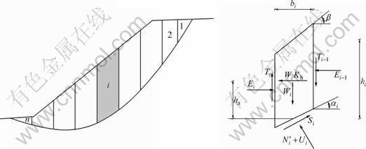
Fig.1 Forces acting on typical slice of natural slope

Consider the summation of moments about the center point of the base of the i-th slice. After simplifying, the moment equilibrium equation is derived in the form of an explicit expression for the scaling factor as

                          (8)

To solve the factor of safety, first specify the form of the inter-slice function f(x) and assume the initial values for F_S and λ. As suggested by ZHU et al [11], the appropriate choice for initial values of F_S and λ are 1 and 0, respectively. Then, F_S is obtained by an iterative procedure. After that, the values of E_i and λ are calculated based on Eqs.(2) and (8). Finally, the factor of safety is recalculated with these computed values of scaling factor. The iterative procedure is completed when the difference between computed values of F_S and λ is within an acceptable tolerance.

3 Probabilistic slope stability analysis

Generally, the factor of safety obtained by the deterministic method is not a consistent measure of safety because various uncertainties are not considered. Therefore, the probabilistic approach has been introduced as an alternative tool for analyzing the safety of earth slope in which various soil parameter uncertainties can be considered rationally. In this approach, safety of a slope is measured by the reliability index (β) or by the probability of failure (P_f), instead of by the classical factor of safety. In a probabilistic analysis, the failure-safety state of a slope may be expressed by the so-called performance function G(X), where X=[X₁, X₂, X₃, …, X_n] denotes the vector of basic random variables of a slope. The performance function partitions the vector space X into two separate regions: the safety region indicated by G(X)>0, and the failure region indicated by G(X)<0, while the limit state surface is presented by G(X)=0. In general, the performance function is a function of the factor of safety (F_S) of a slope which is defined as

G(X)=F_S(X)–1                                                               (9)

The probability of failure may be expressed as

                     (10)

where f_X(X) represents the joint probability density function of the vector of random variables, and the integral is carried out over the failure domain. Consequently, the probability of safe performance, or the reliability of the slope is given by

R=P[G(X)>0]=1–P_f                                                                                         (11)

The performance function, as defined by Eq.(9), is a function of several random variables. To determine the reliability (or the probability of failure), the probability density function of the performance function must be evaluated. This requires multiple integration of the joint probability density function of the random variables over the entire safe (or failure) domain. The joint probability density function of the random variables is generally not well-defined, and the performance function is very implicit. Hence, evaluating the probability density function of the performance function is often not possible. In addition, even if the joint probability density function of the random variables can be specified, the multi-dimensional integral in Eq.(10) usually cannot be solved analytically, and numerical approaches are often required to find the solution. To overcome these difficulties, the reliability index (β) is developed to calculate the competitive reliability of a slope.

HASOFER and LIND [3] proposed a modified definition of the reliability index which is defined as the minimum distance from the origin of normalized basic variables to the limit state (failure) surface. The mean and standard deviations of the normalized variable, z_i, are zero and unity, respectively. The method suggested by HASOFER and LIND [3] is referred to as advanced first-order second-moment (AFOSM) method, and random variables are described only by their first and second statistical moments (i.e., mean, variance and correlation characteristics). To calculate the reliability index defined by HASOFER and LIND (β_HL), all the random variables (X) should be transformed into a standard normal space (Z) as

z_i=(x_i-μ_i)/σ_i                                                                                                               (12)

where μ_i and σ_i represent the mean and the standard deviation of x_i, respectively. According to the transformation in Eq.(12), the mean value point in the X-space (original space) is mapped into the origin of the Z-space (normal space). The failure surface G(X)=0 in X-space is mapped into the equivalent failure surface G(Z)=0 in Z-space, as shown in Fig.2. Figure 2 also shows the concept of reliability index and the most probable point (MPP) of failure for a two-variable case in the standard normal space.

The formulation of the HASOFER and LIND (HL) reliability index (β_HL) is defined in the following form [16-17]:

                                                (13)

where F is the failure domain, Z is a vector representing the set of normalized random variables, and R^-1 is the inverse of the correlation matrix. Mathematically, R=[ρ_ij] (i, j=1, 2, …, n) is a square matrix that contains the correlations between a set of n random variables. Although the correlation coefficient among two random variables has a range of -1<ρ_ij<1, one is not totally free in assigning any value within this range for the correlation matrix. It must be emphasized that the correlation matrix has to be positive definitely [18].

Evaluation of the HL reliability index (β_HL) using the classical method is not possible, especially when correlated non-normal random variables are involved. The reliability index may be calculated using an optimization approach, in which the objective function is the β_HL defined in Eq.(13) and implicit equality constraint defined as the limit state function (G(Z)=0):

                                                 (14)

Or equivalently solve the relaxed form obtained by the penalty method as

                                           (15)

The parameters r and l are problem-dependent, and r should be a suitably large positive constant. In the present study, the values set for r and l are 1 000 and 2, respectively. The solution of the optimization problem in Eq.(14) or Eq.(15) is the reliability index and design point or MPP in the standard normal space. Consequently, the failure probability (P_f) may be evaluated using the established equation as

                                       (16)

where Φ is the standard normal cumulative distribution function. Several algorithms have been proposed for the solution of the optimization problem in Eq.(15) in Ref.[19]. In the current research, a hybrid heuristic optimization algorithm based on chaotic particle swarm optimization and harmony search is proposed for the solution.

4 Hybrid algorithm based on CPSO and HS

4.1 Chaotic particle swarm optimization (CPSO)

Particle swarm optimization (PSO) is a population- based optimization technique introduced by KENNEDY and EBERHART [4] to solve the unconstrained optimization problem. In a PSO system, multiple candidate solutions coexist and collaborate simultaneously. Each solution called a particle, flies in the problem search space looking for the optimal position to land. A particle, during the generations, adjusts its position according to its own experience as well as the experience of neighboring particles. PSO system combines local search method (through self experience) with global search methods (through neighboring experience), attempting to balance exploration and exploitation. A particle status on the search space is characterized by two factors: its position (X_i) and velocity (V_i). The new velocity and position   of particle will be updated according to the following equations [20]:

                      (17)

                                        (18)

where V_i=[v_i,1, v_i,2, …, v_i,n] is called the velocity for particle i, which represents the distance to be traveled by this particle from its current position; X_i=[x_i,1, x_i,2, …, x_i,n] represents the position of particle i; w is called the inertia weight that controls the impact of previous velocity of particle on its current one; p represents the best previous position of particle i (i.e., local-best position or its experience); g represents the best position among all particles in the population X=[X₁, X₂, …, X_N] (i.e. global-best position); Rand(?) and rand(?) are two independently uniformly distributed random variables with range [0, 1]; c₁ and c₂ are positive numbers called acceleration coefficients that guide each particle toward the individual best and the swarm best positions, respectively.

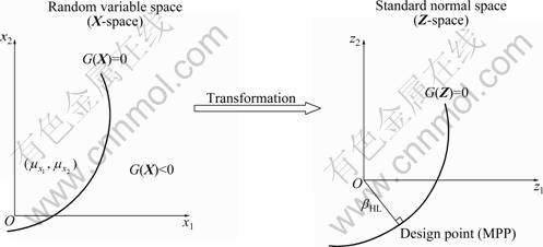
Fig.2 Geometrical representation of definition of reliability index

The inertia weighting function in Eq.(17) is usually evaluated utilizing the following equation:

                                        (19)

where w_max and w_min are the maximum and minimum values of w, k_max is the maximum number of iteration and k is the current iteration number.

Generally, the performance of basic PSO depends nearly entirely on its parameters. The algorithm is usually trapped in local optima in early iterations and suffers from the premature convergence when facing a complex optimization problem. In this work, chaos is inserted into PSO to construct a chaotic PSO (CPSO) and solve the premature convergence problem. The chaotic sequence is capable of improving the global seeking ability of the PSO algorithm and preventing the early convergence to local minima. One of the dynamic systems showing a chaotic manner is a logistic map [21], whose equation is described as

                       (20)

where μ is a control parameter and has a real value in the range of [0, 4], and k is the iteration number. The behavior of the system represented by Eq.(20) is greatly changed with the variation of μ and displays chaotic dynamics when μ=4.0 and θ[1]{0, 0.25, 0.5, 0.75, 1}. The new equation for inertia weight obtained by multiplying Eq.(19) and Eq.(20) reads as

                                                                   (21)

Despite the conventional inertia, the weight decreases monotonously and linearly from w_max to w_min, and the new inertia weight decreases and oscillates simultaneously for the total iteration.

4.2 Harmony search algorithm (HS)

GEEM et al [5] developed a harmony search meta- heuristic algorithm which is based on the natural musical performance process of searching for a perfect state of harmony, such as during jazz improvisation. Generally, the optimization procedure based on the harmony search algorithm may be illustrated as follows:

Step 1: Initialize optimization problem and algorithm parameters

The HS parameters include the number of solution vectors in the harmony memory or the harmony memory size (HMS), harmony memory considering rate (HMCR), pitch-adjusting rate (PAR), and the maximum number of improvisations (K), or termination criterion. These parameters are selected depending on the problem.

Step 2: Initialize harmony memory (HM)

In this step, the harmony memory (HM) matrix as shown in Eq.(22) is randomly generated and sorted by the values of the objective function:

          (22)

where X¹, X², …, X^HMS and f(X¹), f(X²), …, f(X^HMS) show each solution vector for design variables and the corresponding objective function value, respectively.

Step 3: Improvise new harmony from HM

A new harmony vector [x^nh]=[x₁^nh, x₂^nh, …, x_N^nh] is improvised from either the HM or the entire section list. The new harmony vector is generated by three rules: memory consideration, pitch adjustment and random generation.

In the memory consideration process, the value of the first design variable  for the new vector is chosen from any value in the specified HM range   Values of the other decision variables  are chosen by the same rationale. Here, the possibility that a new value will be chosen is indicated by the HMCR parameter, which varies between 0 and 1 as follows:

        (23)

where r is a random number from interval [0,1]. At first, a random number (r) is generated. If this random number is less than the HMCR value, the i-th design variable of the new design [x^nh] is selected from the current values stored in the i-th column of HM. If r is higher than HMCR, the i-th design variable of the new design [x^nh] is selected from the entire section list X_i.

After that, every component of the new harmony vector,  evaluated by memory consideration, is examined to determine whether it should be pitch adjusted. This procedure uses the PAR parameter. PAR investigates better design in the neighboring of the current design and is applied as follows:

Pitch adjusting decision for

                                     (24)

A random number (r) uniformly distributed over the interval [0,1] is generated for x_i^nh. If this random number is less than the PAR, x_i^nh is replaced with its neighboring values. If this random number is not less than the PAR, x_i^nh remains the same. If the pitch adjustment decision for x_i^nh is Yes, the pitch adjustment value of x_i^nh for continuous design variable is

x_i^nhfx_i^nh+α                                                                   (25)

where α is the value of bu(-1, 1); b is an arbitrary distance bandwidth for the continuous variable; and u(-1, 1) is a uniform distribution between -1 and 1.

Step 4: Fitness measure and update harmony memory

In this step, if the new harmony vector, [x^nh]=   is better than the worst design in the HM in terms of the objective function value, the new design is included in the HM, and the existing worst harmony is excluded from the HM. The HM is sorted again by the objective function value.

Step 5: Termination criterion

Repeat Steps 2 and 3 until the termination criterion is satisfied.

4.3 Hybrid CPSO-HS

Hybrid chaotic particle swarm optimization with harmony search algorithm (CPSOHS) results from combining CPSO and HS. The HS algorithm provides a new way to produce new particles. Unlike other heuristic methods, the HS algorithm generates a new design vector considering all existing design vectors. Furthermore, to improve the global optimum prediction and to allow the solution escape from local optima, the HMCR and PAR parameters are implemented by HS algorithm. Because of these advantages, in this work, the HS concept has been incorporated into the CPSO to find each solution in all dimensions and to explore the potential solution space. In this approach, all the particles are regarded as HM and the dimension of particle is HMS. In the proposed CPSOHS, the new harmony (particle) improvises utilizing the HS algorithm by considering all the harmonies (particles) at each iteration. If the new produced harmony is better than the worst harmony (according to the fitness value), the worst harmony will be replaced by the newly produced harmony. The framework of CPSOHS for the reliability assessment of earth slope is presented as a flowchart in Fig.3. One of the major advantages of the proposed CPSOHS is preventing premature convergence, especially in heavily constrained and handling problems with more local optima.

5 Example analysis and results

The applicability and validity of the proposed CPSOHS algorithm to reliability assessment of earth slope will be investigated by considering a number of published cases. The implementation of the proposed methodology for the reliability analysis of the earth slope is shown as a flowchart in Fig.3. The procedure has been carried out using a computer program that was developed in MATLAB. The program is capable of searching for the minimum factor of safety and reliability index and the most critical deterministic and probabilistic slip surface of earth slope. To apply CPSOHS for the reliability analysis of earth slope, the parameters of the algorithm should be adopted accurately. In the present study, proper fine-tuning of the parameters is carried out utilizing several experimental studies examining the effect of each parameter on the final solution and convergence of the algorithm. As a result, a population of 30 individuals was used; w_max and w_min were chosen as 0.9 and 0.45, respectively; c₁ and c₂ were selected equal to 2; the control parameter (μ) was set to 4.0 and θ[1] was considered as 0.55; the harmony memory consideration rate (HMCR) was considered as 0.8 and pitch-adjusting rate (PAR) was set equal to 0.3. Finally, a fixed number of maximum iteration (k_max) of 4000 was applied. The optimization procedure will be terminated when the maximum iteration number is reached or the best solution does not improve after a given number of iterations.

5.1 Example 1: Application to homogeneous slope

The first case is a homogeneous slope with height of 10 m and the slope inclination of 18.4°, which was studied earlier by CHOWDHURY and XU [22]. The cross section and the geometry of a slope are presented in Fig.4.

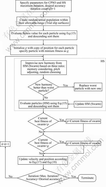
Fig.3 Flowchart of CPSOHS algorithm for reliability analysis of slopes

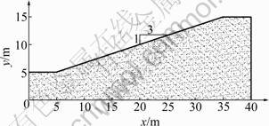
Fig.4 Cross section of homogeneous slope – Example 1

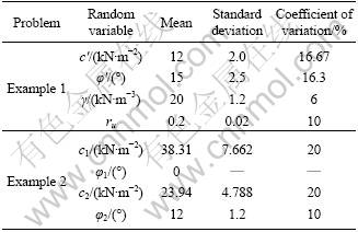
In this case, the effective friction angle (φ'), effective cohesion (c'), unit weight (γ) and pore water pressure ratio (r_u) are considered as random variables. The first and second statistical moments (i.e. mean and standard deviation) of the random variables are presented in Table 1. In this example, all the random variables are assumed to be normally distributed, and three cases will

be considered for analysis, based on correlation between random variables as follows:

Case 1: Uncorrelated random variables with r_u=0;

Case 2: Correlated random variable with ρ_cφ=-0.3, ρ_cγ=0.4 and ρ_φγ=0.7;

Case 3: Correlated random variable with ρ_cφ=0.5, ρ_cγ= 0.4 and ρ_φγ=0.7.

CHOWDHURY and XU [22] solved the problem and evaluated both the minimum factor of safety and the HASOFER and LIND reliability index. The results of the proposed CPSOHS method and their study are summarized in Table 2. Moreover, to verify the accuracy and efficiency of the proposed method, the result of PSO is also presented. In Table 2, F_S,min and β_min are the minimum factor of safety and the minimum HL reliability index associated with the critical deterministic and probabilistic slip surface, respectively. From  analyzing the results, it can be observed that the minimum reliability indexes calculated using the presented CPSOHS method for all three cases are lower than the values reported by CHOWDHURY and XU [22] and also PSO. Further, the minimum factors of safety calculated from a deterministic analysis based on the mean values of the soil properties obtained by CPSOHS are lower than those reported by CHOWDHURY and XU [22] and slightly lower than those achieved by PSO.

Table 1 Statistical properties of soil parameters – Examples 1 and 2

From Table 2, it is also clear that the reliability index is sensitive to the correlation coefficient between random variables, in which β_min decreases as the value of ρ_cφ increases. Moreover, the reliability (or probability of failure) of slopes is sensitive to the variation of soil strength. The effects of these parameters on the reliability of earth slope are investigated by running a set of sensitivity studies using the presented procedure. For this purpose, the third case (ρ_cφ=0.5, ρ_cγ= 0.4 and ρ_φγ=0.7) is reconsidered as a basic case. Each variable allowed varying independently about its respective mean value, while the other properties were kept fixed at their mean values. Further, the coefficient of variation (COV) values of mentioned parameters is allowed to change. Figures 5(a) and 5(b) show the relationships between the reliability index, effective friction angle and effective cohesion of soil. Figures 5(a) and 5(b) show how the reliability index may be affected by the uncertainty in soil strength. These figures illustrate that an increase in mean of c′ and φ′ leads to the increase of the reliability index (or decrease of P_f). Also, it can be seen that the reliability index could be decreased when the COV of c′ and φ′ increases, and for a relatively large value of these parameters, the reliability is significantly sensitive to the COV of soil strength.

Moreover, to investigate the influence of the probability distribution type on the estimated reliability index, the first case (uncorrelated random variables with r_u=0) is considered, and all the random variables are assumed to be characterized statistically by a normal and lognormal distribution. In such a case, the COV values of soil properties (c′, φ′ and γ) are varied from their corresponding base case to their upper bound values, according to v_φ=0.1+0.2ζ, v_c=0.2+0.3ζ, and v_γ=0.01+ 0.09ζ for ζ ranging from 0 to 1. The ranges of the COV values are in agreement with those suggested by PHOON and KULHAWY [23]. The reliability indexes obtained by considering that all the random variables are normally or lognormally distributed are shown in Fig.6. From the results presented in Fig.6, it is clear that the reliability indexes evaluated with the assumption of normally distributed random variables are slightly lower than those calculated with lognormally distributed variables. Because of the lognormal distribution, the variables are not permitted to take negative values. Moreover, as shown in Fig.6, the reliability index decreases when the COV values of soil properties increase. The results also show that as the reliability index becomes small, it is less sensitive to the distribution type assumption.

Table 2 Results comparison – Example 1

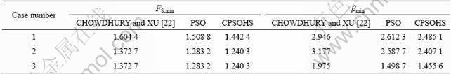
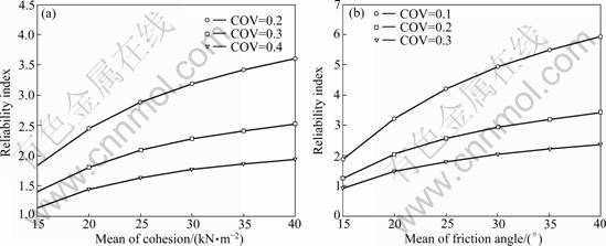
Fig.5 Variations of reliability index with different values of soil strength: (a) Reliability index for different values of cohesion;     (b) Reliability index for different values of friction angle

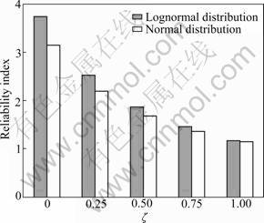
Fig.6 Variations of reliability index with COV for normal and lognormal random variables

5.2 Example 2: Application to two-layered slope

This example considers a two-layered slope in clay bounded by a hard layer below and parallel to the ground surface with a cross section, as shown in Fig.7. The soil strength parameters that are related to the stability of slope, including friction angle φ and cohesion c, are considered as random variables. The random variables are assumed to be uncorrelated and have normal distributions. The statistical moments (mean value and standard deviation) of the parameters are summarized in Table 1.

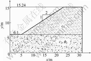
Fig.7 Cross section of non homogeneous slope – Example 2

This example was studied earlier by HASSAN and WOLFF [24], BHATTACHARYA et al [25], XU and LOW [26], and CHOWDHURY and RAO [27]. The results obtained from the current study, together with a comparison of those reported by previous researchers, are summarized in Table 3. For the results shown in Table 3, it can be assumed that the minimum reliability index evaluated using CPSOHS is 2.043, which is almost lower than those reported by others and also PSO (2.106). Besides, the minimum factor of safety calculated by the presented method is lower than that reported by the other researchers.

Table 3 Results comparison – Example 2

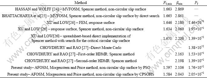
Figure 8 presents the convergence characteristics of the PSO and CPSOHS methods for the calculation of the minimum reliability index. From Fig.8 and also Table 3, it can be concluded that in addition to generating superior results, the CPSOHS has a very fast convergence rate in the early iterations and performs significantly better than the PSO.

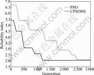
Fig.8 Convergence characteristics of proposed CPSOHS and PSO – Example 2

Similar to the first example in this case, the influence of the probability distribution type on the estimated reliability index is examined by considering that all the random variables have a normal and lognormal distribution. In this example, the COV values of soil properties (c′ and φ′) are varied from their corresponding base case to their upper bound values, according to v_φ=0.1+0.2ζ and v_c=0.2+0.3ζ for ζ ranging from 0 to 1. Figure 9 presents the variation of reliability indexes by considering that all the random variables are normally or lognormally distributed. As can be seen from Fig.9, the reliability indexes evaluated with normal basic variables are slightly lower than those calculated with lognormal variables. The presented results show that, as the COV values of soil properties increase, β decreases. The results also show that the reliability index becomes relatively insensitive to the assumption of the distribution type when the COV values of soil properties increase.

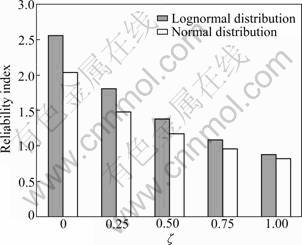
Fig.9 Variations of reliability index with COV for normal and lognormal random variables

5.3 Example 3: Application to a case study of Cannon Dam

In this example, the reliability analysis for the end- of-construction stage of the Cannon Dam reported by HASSAN and WOLFF [24] will be investigated. A typical cross section and the geometry of the dam showing the soil profile is presented in Fig.10.

The structure consists of two zones of compacted clay: Phase I fill and Phase II fill over layers of sand and limestone. Strength parameters of the two clay layers were considered as random variables (c₁, φ₁, c₂, φ₂) and all random variables are assumed to have a lognormal distribution. The mean value, standard deviation, COV and correlation coefficient for these parameters based on UU tests of recorded samples from the embankment are shown in Table 4 [24]. HASSAN and WOLFF [24] made no reductions in the variance for spatial correlation. In their study, it was conservatively assumed that variance over a failure zone was potentially as large as the point variance.

The minimum reliability index and factor of safety corresponding to the critical probabilistic and deterministic slip surface obtained by different methods are shown in Table 5. As derived from Table 5, the minimum factor of safety evaluated by the presented analysis method (2.564) is slightly lower than that evaluated by the other methods. As it can be derived from Table 5, the reliability index evaluated herein is lower than that reported in the previous study and also PSO.

Fig.10 Cross section of Cannon Dam – Example 3

Table 4 Statistical properties of soil parameters – Example 3

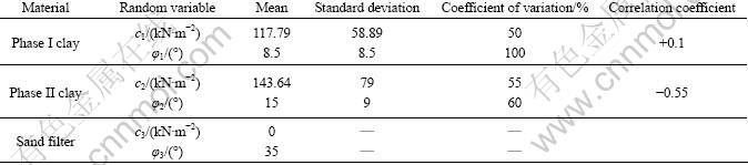
Table 5 Results comparison – Example 3

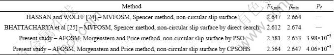
Figure 11 shows the convergence history of the minimum reliability index evaluated by PSO and CPSOHS algorithms. As can be seen from Fig.11 and also Table 5, the proposed algorithm requires far fewer iterations, and it is better than the PSO in terms of accuracy and convergence speed.

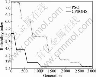
Fig.11 Convergence characteristics of proposed method and PSO – Example 3

6 Conclusions

1) An effective numerical procedure for reliability analysis of earth slope is developed, built upon the advanced first-order second-moment (AFOSM) method and a new approach of the Morgenstern and Price method of slices.

2) The problem of searching the minimum reliability index associated with the critical probabilistic failure surface of slopes is formulated as an optimization problem and a hybrid heuristic optimization method based on chaotic particle swarm optimization and harmony search algorithm (CPSOHS) is proposed for the solution.

3) The advantages of the proposed CPSOHS algorithm are obviously demonstrated through three numerical examples from the literature. Comparison of the results shows that the proposed method calculates smaller values of the reliability index and factor of safety and generates superior results in terms of accuracy and convergence rate.

4) From the sensitivity analysis preformed herein, it is found that the cohesion and the angle of friction of soil have a direct relationship with the reliability index, in which, as the mean of these parameters increases, the reliability index increases.

5) As the coefficient of variation (COV) of soil strength increases, the reliability index decreases (or probability of failure increases), especially for large values of soil strength parameters.

6) The sensitivity analysis shows that the assumed or adopted probability distribution types for the random variables may affect the reliability of slopes. The results demonstrate that the reliability indexes evaluated with normally distributed random variables are slightly lower than those calculated with lognormally distributed variables, and conservative results will be evaluated by considering a normal distribution for random variables.

Acknowledgements

The research reported herein is supported by the Ministry of Higher Education, Malaysia (Grant No. UKM-AP-PLW-04-2009/2). This support is gratefully acknowledged.

References

[1] ANG A H S, TANG W H. Probability concepts in engineering planning and design, Vol. 2—Decision, risk, and reliability [M]. New York: Wiley, 1984: 333-346.

[2] CHRISTIAN J T, LADD C C, BAECHER G B. Reliability applied to slope stability analysis [J]. Journal of Geotechnical Enggineering, 1994, 120(12): 2180-2207.

[3] HASOFER A, LIND N. Exact and invariant second-moment code format [J]. Journal of Engineering Mechanics, 1974, 100(1): 111-121.

[4] KENNEDY J, EBERHART R C. Particle swarm optimization [C]// Proceeding of the IEEE international conference on neural networks. Perth, Australia, 1995: 1942-1948.

[5] GEEM Z W, KIM J H, LOGANATHAN G V. A new heuristic optimization algorithm: Harmony search [J]. Simulation, 2001, 76(2): 60-68.

[6] CHENG Y M, LI L, CHI S C, WEI W B. Particle swarm optimization algorithm for the location of the critical non-circular failure surface in two-dimensional slope stability analysis [J]. Computers and Geotechnics, 2007, 34(2): 92-103.

[7] CHENG Y M, LI L, CHI S C. Performance studies on six heuristic global optimization methods in the location of critical slip surface [J]. Computers and Geotechnics, 2007, 34(6): 462-484.

[8] CHENG Y M, LI L, LANSIVAARA T, CHI S C, SUN Y J. An improved harmony search minimization algorithm using different slip surface generation methods for slope stability analysis [J]. Engineering Optimization, 2008, 40(2): 95-115.

[9] LI L, YU G M, CHEN Z U, CHU X S. Discontinuous flying particle swarm optimization algorithm and its application to slope stability analysis [J]. Journal of Central South University of Technology, 2010, 17(4): 852-856.

[10] MORGENSTERN N R, PRICE V E. The analysis of the stability of general slip surfaces [J]. Geotechinque, 1965, 15(1): 79-93.

[11] ZHU D Y, LEE C F, QIAN Q H, CHEN G R. A concise algorithm for computing the factor of safety using the Morgenstern–Price method [J]. Canadian Geotechnical Journal, 2005, 42(1): 272-278.

[12] BISHOP A W. The use of the slip circle in the stability analysis of earth slopes [J]. Geotechinque, 1955, 5(1): 7-17.

[13] SPENCER E. A method of analysis of the stability of embankments assuming parallel inter-slice forces [J]. Geotechnique, 1967, 17(1): 11-26.

[14] JANBU N. Slope stability computations: Embankment dam engineering [M]. New York: John Wiley, 1973: 47-87.

[15] FREDLUND D G, KRAHN J. Comparison of slope stability methods of analysis [J]. Canadian Geotechnical Journal, 1977, 14(3): 429-439.

[16] DITLEVSEN O. Uncertainty modeling with applications to multidimensional civil engineering systems [M]. New York: McGraw-Hill, 1981: 245-290.

[17] LOW B K, TANG W H. Reliability analysis of reinforced embankments on soft ground [J]. Canadian Geotechnical Journal, 1997, 34(5): 672-685.

[18] LOW B K, TANG W H. Reliability analysis using object-oriented constrained optimization [J]. Structural Safety, 2004, 26(1): 69-89.

[19] LIU P L, KIUREGHIAN A D. Optimization algorithms for structural reliability [J]. Structural Safety, 1991, 9(3): 161-177.

[20] SHI Y H, EBERHART R C. A modified particle swarm optimizer [C]// IEEE World Congress on Evolutionary Computation. Anchorage, Alaska, 1998: 69-73.

[21] MAY R M. Simple mathematical models with very complicated dynamics [J]. Nature, 1976, 261: 459-467.

[22] CHOWDHURY R N, XU D W. Reliability index for slope stability assessment-two methods compared [J]. Reliability Engineering and System Safety, 1992, 37(2): 99-108.

[23] PHOON K K, KULHAWY F H. Characterization of geotechnical variability [J]. Canadian Geotechnical Journal, 1999, 36(4): 612-624.

[24] HASSAN A M, WOLFF T F. Search algorithm for minimum reliability index of earth slopes [J]. Journal of Geotechnical and Geoenvironmental Engineering, 1999, 125(4): 301-308.

[25] BHATTACHARYA G, JANA D, OJHA S, CHAKRABORTY S. Direct search for minimum reliability index of earth slopes [J]. Computers and Geotechnics, 2003, 30(6): 455-462.

[26] XU B, LOW B K. Probabilistic stability analyses of embankments based on finite-element method [J]. Journal of Geotechnical and Geoenvironmental Engineerin, 2006, 132(11): 1444-1454.

[27] CHOWDHURY R, RAO B N. Probabilistic stability assessment of slopes using high dimensional model representation [J]. Computers and Geotechnics, 2010, 37(7/8): 876-884.

(Edited by YANG Bing)

Received date: 2010-11-30; Accepted date: 2011-03-29

Corresponding author: M. Khajehzadeh; Tel: +60-173207611; E-mail: mohammad.khajehzadeh@gmail.com