
Trans. Nonferrous Met. Soc. China 24(2014) 597-604
Applications of nonferrous metal price volatility to prediction of China��s stock market
Die-feng PENG, Jian-xin WANG, Yu-lei RAO
Institute of Metal Resources Strategy, Central South University, Changsha 410083, China
Received 10 August 2013; accepted 25 September 2013
Abstract:
The aim of the present work is to examine whether the price volatility of nonferrous metal futures can be used to predict the aggregate stock market returns in China. During a sample period from January of 2004 to December of 2011, empirical results show that the price volatility of basic nonferrous metals is a good predictor of value-weighted stock portfolio at various horizons in both in-sample and out-of-sample regressions. The predictive power of metal copper volatility is greater than that of aluminum. The results are robust to alternative measurements of variables and econometric approaches. After controlling several well-known macro pricing variables, the predictive power of copper volatility declines but remains statistically significant. Since the predictability exists only during our sample period, we conjecture that the stock market predictability by metal price volatility is partly driven by commodity financialization.
Key words:
commodity futures; nonferrous metals; price volatility; stock return; predictability;
1 Introduction
The world commodity market has witnessed a big metal price boom in the last decade. Metal prices have risen to recorded nominal highs since the turn of the millennium. According to the data from LME, among all the six Commodity Research Bureau (CRB) categories of primary commodities, metals experienced the greatest dramatic price fluctuation in the 2002-2008 commodity boom. Especially in the commodity market collapse during the financial crisis, the prices of basic metals fell 60%-75% from the peak to the bottom.
The integration of metal prices fluctuation with macroeconomic business cycles and financial market has been of recent interest. Labys et al [1] documented that the commonality in metal prices reflects the tendency of commodity markets to respond to common business cycles and trend factors. The common factors in metal price can be related to macroeconomic influences, such as industrial production, consumer prices, interest rates, stock prices, and exchange rates. A more recent work by Chen [2] investigated the time-serial properties of the prices of 21 metals and found that 34% of price volatility can be attributed to global macroeconomic factors over the period of 1972-2007. A large body of empirical evidence suggested that the commodity index investment was the major driver of the current spike in commodity futures, aggravating the integration of commodity market and financial market in the process of financialization [3-8].
The trade-off between risk and expected return is essential in any equilibrium theory of finance. From an aggregate perspective, as systematic risk increases, risk-averse investors require a higher risk premium to hold aggregate wealth, and the equilibrium expected return must rise. However, the questions posted are that the systematic risks are unobserved. Although the measure of stock market variance is thought to be a proxy of systematic risk, stock market volatility may itself be poor forecast of future stock market returns [9]. According to the trading data from 2004 to 2011 in the commodity markets in China, metal futures, such as copper and aluminum, attract the greatest interest of speculation and hedge trading, with its price fluctuating with sorts of macro shocks. Since commodity risk begins to be regarded as part of the macro risk source, it is intuitive to take commodity price volatility into our consideration to proxy systematic risk. Can the volatility of metal prices predict the aggregate stock market returns in China since the emergence of commodity financialization?
To find the answer to the question above, we collect the data from China��s metal futures and stock market and examine whether there is a substantial predictive relationship between lagged metal volatility and aggregate stock market returns. For the availability of data, we choose two typical nonferrous metals, copper and aluminum, as representatives of all kinds of metals on the commodity market. In-sample and out-of-sample regression results show that the volatilities of copper and aluminum are capable of forecasting stock market return at various horizons, which is consistent with our conjecture. Additionally, the results remain stable after controlling several well-known macro-economic variables and are quantitatively similar by alternative measurement of variables. However, the predictive significance loses when we replicate our results at an earlier period from 1995 to 2003, which lends part of the predictability in our sample period to the prevailing commodity financialization.
The work contributes to the literature on metal volatility. A large amount of them study the volatility of precious metals [10-15]. A few of them [16-19] focus on the time-series property of industrial metals volatility, especially the spillover effect between commodity markets and the financial markets. COCHARN et al [19] showed that the implied volatility of the stock return plays a significant role in determining metal risk and return. In the present work, authors attempt to examine the forecasting power of metal volatility, through a standard procedure of predicting stock returns, instead of complex time-series model using high-frequency data.
2 Methodology
To analyze the predictability of metal volatility for stock market return, we run monthly long-horizon predictive regressions as follows:
 (1)
(1)
where rt+1, t+K is the continuously compounded return measured over K months in the future, and xt is a forecasting variable known at time t. The forecasting horizons are 1, 3, 6, 9 and 12 months ahead.
The statistical inference for the slope estimates is based on both asymptotic t-statistics and empirical p-values obtained by NEWEY and WEST [20] from a Bootstrap experiment [21]. This bootstrap simulation produces an empirical distribution for the estimated predictive slopes that should represent a better approximation of the finite sample distribution of these estimates. In this simulation, the market return and the forecasting variables are simulated (10000 times) under the null of no predictability of the market return.
First, estimate the original regression Eq. (1) using ordinary least squares (OLS), save the slop estimate  : and assume that the predictor, xt, follows an AR(1) process and estimate Eqs. (2) and (3)
 (2)
(2)
 (3)
(3)
The time-series of OLS residuals,  and
and  , and the OLS estimates,
 ,
,  ,
,  are saved. In each replication, m=1, ��, 10000, the pseudo-samples for the innovations in the market return and the predictor are constructed by drawing with replacement from the two residuals:
 (4)
(4)
 (5)
(5)
The time indices  are created randomly from the original time sequence, 1, ��, T. The innovations in both the return and predicator have the same time sequence to account for their contemporaneous cross-correlation. For each replication, m=1, ��, 10000, a pseudo-sample of the market return and predictor are constructed
 (6)
(6)
 (7)
(7)
Use the artificial data rather than the original data to estimate the following equation:
 (8)
(8)
The initial value for xt(x0) is picked at random from one of the observations of xt. In result we get an empirical distribution of the regression slope estimates, 
 (9)
(9)
where denotes the number of bootstrapped slop estimates that are higher than the absolute of original slop estimate.
GOYAL and WELCH [22] suggested that most forecasting variables with in-sample forecasting power do not demonstrate an ability to forecast returns out-of-sample. Following CAMPBELL and WELCH [23], GOYAL and THOMPSON [22], GUO [24], RAPACH et al [25] and FERREIRA et al [26], we use  to test the out-of-sample predictability.
The is calculated as
 (10)
(10)
where Rt is the real market return of time t,  is predicted by a model which is from a regression estimated through period t-1,
  is the historical average return estimated through period t-1, and n is the starting point we try to predict.
If >0, then the out-of-sample prediction has lower average mean-squared prediction error (MSPE) than the historical average return, which means it has good out-of-sample predictability. To test whether the average mean-squared prediction error of the out-of-sample prediction is significantly lower, we use MSPE-adjusted [27] statistic calculated as
 (11)
(11)
where Rt is the real market of time t, t��[1, ��, T]. Then regress  on a constant and use the t-statistic of the constant to test if >0 is significant.
3 Data
We would like to highlight the role of financialization in the prediction of aggregate stock market return. Consequently, we choose the year of 2004, considered to be the beginning of commodity financialization as the start year of our sample period. Therefore, the entire sample period of our analysis is from January of 2004 to December of 2011, 84 months in total. We choose copper and aluminum to represent the family of metal futures for a couple of reasons. First, copper and aluminum, as basic nonferrous metal categories, play a fundamental role in manufacture, architecture and other industries, expected to have more universal impact on the stock market. Second, copper and aluminum are the first sorts of tradable commodities in China��s commodity future market, with the price data available since the earlier of 1990s. Other metals, such as iron, silver, gold, zin, and lead, are not allowed to be traded until recent years. Besides the advantage of data availability, the trading volume of future copper is of extremely great magnitude. According to the data provided by Shanghai Future Exchange, the trading volume of copper in 2012 has exceeded 29 trillion RMB until the end of October, which accounts for 60% trading volume of the entire metal commodity future market. During the first ten months, in contrast, the trading volume of the aluminum market comes to be only 537.93 billion, approximately 1% of the whole metal market.
To predict the stock market, our dependent variable is the value weighted stock portfolio returns of the entire universe of A-share firms listed on Shanghai or Shenzhen stock markets in China, which is denoted by SM_RET. The independent variable we construct to forecast the stock market is the volatility of copper or aluminum. The volatility of copper (CU_VOL) in each month is calculated by the standard deviation of the future copper daily price changes of all trading days during this month. The volatility of aluminum (AL_VOL) is measured in a similar way.
According to the existent empirical work on stock market prediction, we need to control for additional macroeconomic variables in our regression framework. JIANG et al [28] found that five out of twelve well-documented variables at monthly intervals succeed in predicting the aggregate stock market returns in China from 1996 to 2009. The five time-series variables are stock market dividend yield (MDY), market-wide turnover (TURNOVER), inflation index change (INFL), the shock of money supply measure M1 (M1G) and the shock of money supply measure M2 (M2G). The definitions of these five variables are described as follows.
1) Market dividend yield (MDY): difference between the log of dividends and the log of lagged stock prices.
2) Market-wide turnover (TURNOVER): the monthly trading volume over the market value of the whole universe of A-share stocks at the end of the month.
Inflation index change (INFL): Calculated by the monthly difference in CPI index.
3) M1 growth shock (M1G): The first-order difference of the growth in M1 money supply, namely the unexpected shock of M1 supply.
4) M2 growth shock (M2G): The first-order difference of the growth in M2 money supply, namely the unexpected shock of M2 supply.
Figure 1 shows the cumulative returns of three tradable assets, value-weighted stock market index, one-month futures for copper and aluminum in SHFE (Shanghai Futures Exchange), calculated by the holding period gross returns by investing 1 RMB on each of them at the beginning of a sample period. Obviously, the stock market spikes its price in the later of 2007 and then falls down with the coming of global financial crisis. The copper price increases dramatically at the beginning of 2006 and persists on a higher level until the fiercely collapse in the crisis. Apparently, we notice that the price trend of aluminum is almost flat, with similar but much more moderate fluctuations during the sample period. Together with the fact that copper is greatly more heavily traded than aluminum, we conjecture that the price of future copper behaves more like other financial assets rather than aluminum.
We depict the monthly volatility of both metals in Figure 2. In most of cases during the sample period, the curve of copper volatility fluctuates above that of aluminum but with simultaneous oscillation, which tells us that the daily price of copper is more volatile than aluminum. The first peak of both CU_VOL and AL_VOL emerges in the middle of 2006, and the second is at the beginning of 2009, both of which happened to be the start periods of a new upward tendency in the stock market. If it is true, to a certain extent, we speculate that the high volatile metal market might trigger a bullish stock market subsequently through some underlying mechanism.
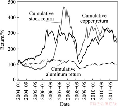
Fig. 1 Cumulative returns of copper, aluminum and stock market index

Fig. 2 Price volatility of copper and aluminum
Table 1 reports the descriptive statistics of major variables. In panel A, we find the values of basic statistics of copper price change (CU_RET) are close to those of stock market return (SM_RET). In contrast, the numeric characteristics of aluminum price change (AL_RET) is quite different from that of both CU_RET and SM_RET. For example, the mean of CU_RET change is 1.426%, very close to the average return of stock market portfolio, which is 1.461% per month, but much greater than that of AL_RET which is only 0.13% per month. The mean of CU_VOL is also greater than that of AL_VOL; nevertheless, the difference, in magnitude, is much smaller than the gap of price change. Besides, the price change of copper and the three volatility variables are rejected by Jarque-Bera statistics to be assumed to follow normal distribution while the normal-distribution assumption about the market portfolio return andaluminum cannot be rejected. We rejected the assumption to have a unit root for all the six variables at the significant level of 1%. All of them are first-order auto-correlated except the stock market return.
Table 1 Summary statistics of main variables
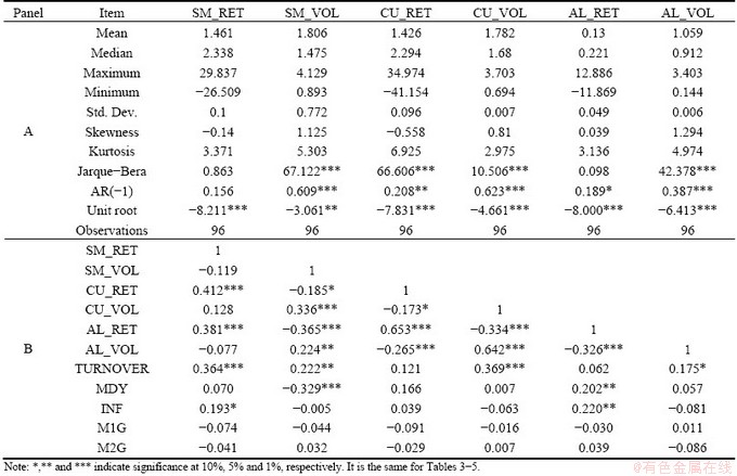
In panel B, we notice that the stock market return is positively correlated with the copper price change as well as the aluminum price change. The correlation coefficients of SM_RET with CU_RET and AL_RET are 0.412 and 0.381 respectively, both at a significant level of 1%. In contrast, the contemporaneous correlations of SM_RET with all the three volatility variables are of no statistical significance. Given the fact of the aggravating co-movements between commodities, the price changes of copper and aluminum, as well as the volatility of them, are highly correlated, with significant coefficients of 0.653 and 0.642 respectively. Besides, the metal volatility variables are both significantly correlated with stock market turnover (TURNOVER) and dividend yield (MDY), while the correlations with three other variables, such as inflation (INF) and the shock of the money supply (M1G and M2G), are negligible in both magnitude and significance.
4 Empirical results
We first examine the predictability of metal volatility for the stock market return in a univariate regression framework. To this end, we regress the market returns at various horizons on the lagged volatility variables of copper and aluminum, using both in-sample and out-of-sample forecasting approaches. Next, we further controll additional variables through multiple predictive regressions and check the robustness of the predictability.
4.1 Univariate test
We present the in-sample predictability results in Table 2. The dependent variables in the regression is the continuously compounded return measured over K months in the future (K=1, 3, 6, 9, 12). The independent variables are one month-lagged copper volatility and aluminum volatility. As the horizon K increases, the coefficient of copper volatility increases monotonically, from 3.608 to 27.871. All the coefficients are at 1% significant level according to the bootstrap p-value except that of the 12-month horizon (t=1.912). Different from the magnitude change of the coefficient, the R-square value changes with an inverse U-shaped trend. The lagged copper volatility succeeds in explaining 14.9% of the 3-month market return variation, which is the highest among all five horizons. The lagged aluminum volatility fails to predict one-month stock market return in any statistical significance levels. However, the predictability of aluminum volatility in longer horizons is as significant as that of copper volatility. Notably, when the forcasting horizon increases to twelve months, the R square increases to 11.3%, which is about twice as high as that of regression on copper volatility.
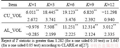
Next, we analyze the out-of-sample (OS) predictive power of copper and aluminum volatility for the stock market return. The OS regressions can be seen as complementary to the in-sample regressions and try to evaluate the parameter instability in these regressions. The out-of-sample predictability results are shown in Table 3. We use 2007 to 2011 as the prediction period while the estimation period is from 2004. The statistic for copper volatility is positive for K=1, 3, 6 and 9, especially for K=3 and 6, statistic is greater than 20%, and all are statistically significant at 5%. For K=12, statistic becomes negative, indicating that the copper volatility cannot predict the stock market return any more for 12 months. For aluminum volatility, the statistic is also positive when K=3, 6, and 9, and is statistically significant at 5%, although it is not great as copper volatility, but still greater than 10% when K=6 and 9. Overall, the out-of-sample results for copper and aluminum volatility to predict stock market return is similar with in-sample results above.
Table 2 In-sample forecasting regressions
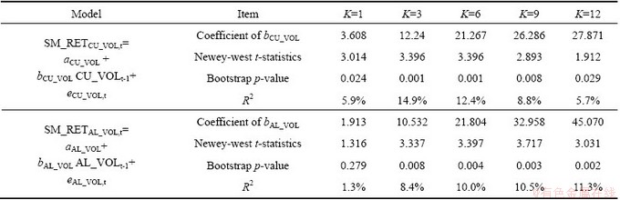
Table 3 Out-of-sample forecasting regressions
4.2 Multivariate regression
The objective of the multivariate regressions is to check whether the forecasting power of metal volatility remains robust in the presence of the alternative predictors. Besides the five variables referred in the section of data description, we continue to control two additional variables: lagged stock market return (SM_RET) and lagged stock market volatility (SM_VOL). The multiple predictability of copper volatility for various horizons is reported in Table 4. All the coefficients of copper volatility in the multivariate regressions are smaller than those of univariate regressions at each horizon, but still statistic significant at 5% or 10% level. For example, the one-month predictive coefficient of CU_VOLt-1 is 3.06 at a significant level of 10% (bootstrap p=0.089), less significant than that of univariate case, in both economic and statistical senses. When the forecasting horizon increases, the coefficient increases monotonically while the bootstrap p value goes first downwards then upwards, in a typical inverse U-shaped trend similar with the univariate case. None of the control variables are statistically significant for short forecasting horizons. As the horizon increases to six months or even longer, the coefficients of SM_RETt-1 and SM_VOLt-1 are becoming significant at 10% level. By adding controls, the gross R2 increases from 5.9% in the univariate regression to 13.8% in the multiple regression when K=1. When the forecasting horizon increases to twelve months, the values of R square increases to an incredibly high level of 56.4%.
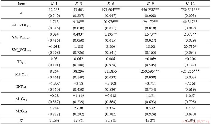
Correspondingly, we report the multivariate regression results of aluminum volatility in Table 5. Similar to the univariate regression, the coefficient of lagged aluminum volatility for one-month forecasting horizon is still insignificant after controlling the lagged market return and volatility and other five macroeconomic variables. However, the coefficient of AL_VOLt-1 goes upward when the forecasting horizon increases and is significant at a level of 5% for other four horizons, where the respective R2 is greater than that of regression on lagged copper volatility.
Table 4 Multiple predictive regressions on lagged copper volatility
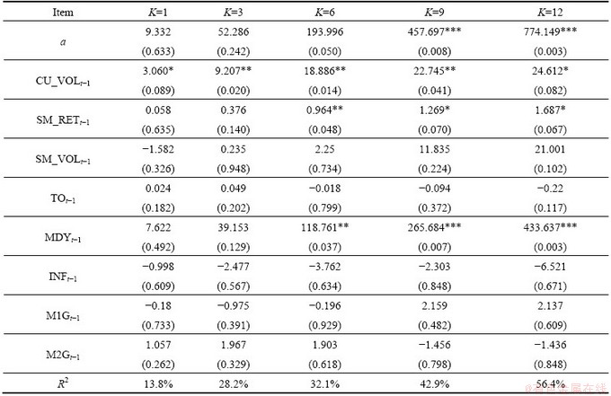
Table 5 Multiple predictive regressions on lagged aluminum volatility
4.3 Robustness test
The dependent variable of our earlier analysis is value-weighted stock portfolio returns of the entire market, we repeat our regressions using China Security Index 300 (CSI 300) as a dependent variable. We also adjust the earlier value-weighted stock portfolio returns of the entire market by excluding the risk-free rate of interest to repeat our analysis. For these two different settings, we find the results are quite similar with earlier analysis and are thus not tabulated here.
The copper and aluminum volatility used earlier is calculated through an one-month period. We repeat our main analysis using three-months copper and aluminum volatility as an independent variable. In untabulated results, we find that the results are also quite consistent with earlier. To save space, all the above tables are not reported but are available upon request.
Finally, we replicate the predictive regressions on another time interval from January of 1995 to December of 2004, a period before commodity financialization. Consistent with our conjecture, we could not observe the similar predictive relationship between lagged metal volatility and stock aggregate stock market return. So we limit our finding to the recent period and leave the possibility of the explanation for the predictability to commodity financialization.
5 Conclusions
1) The price volatility of future copper and aluminum is capable of predicting value-weighted stock portfolio at various horizons in both in-sample and out-of-sample regressions.
2) The basic results are robust after controlling the macroeconomic variables and not influenced by using alternative ways to construct variables and some econometric adjustment.
3) Weak evidence suggests that the discovered predictability is likely to be attributed to the prevailing financialization trend in the recent commodity market.
References
[1] LABYS W C, ACHOUCH A, TERRAZA M. Metal prices and the business cycle [J]. Resources Policy, 1999, 25: 229-238.
[2] CHEN M H. Understanding world metals prices��Returns, volatility and diversification [J]. Resources Policy, 2010, 35: 127-140.
[3] GILBERT C L. Speculative influences on commodity futures prices 2006-2008 [R]. United Nations Conference on Trade and Development, 2010.
[4] GILBERT C L. How to understand high food prices [J]. Journal of Agricultural Economics, 2012, 61: 398-425.
[5] EINLOTH J. Speculation and recent volatility in the price of oil [R]. SSRN Working paper 1488792. 2009.
[6] TANG K, XIONG W. Index investment and financialization of commodities [R]. NBER Working Paper 16385. 2010.
[7] SILVENNOINEN A, THORP S. Financialization, crisis and commodity correlation dynamics [R]. University of Technology SydneyResearch Paper No 267. 2010.
[8] HENDERSON B, PEARSON N, WANG L. New evidence on the financialization of commodity markets [R]. FDIC��s 22nd Annual Derivatives and Risk Management Conference, 2012.
[9] POLLET J M, WILSON M. Average correlation and stock market returns [J]. Journal of Financial Economics, 2010, 96: 364-380.
[10] BATTEN J A, CINER C, LUCEY B M. The macroeconomic determinants of volatility in precious metals markets [J]. Resources Policy, 2010, 35: 65-71.
[11] MOHAMED E, HEDI A, SHAWKAT H, AMINE L, DUC KN. Longmemory and structural breaks in modeling the return and volatility dynamicsof precious metals [J]. The Quarterly Review of Economics and Finance, 2012, 52(2): 207�C218.
[12] HAMMOUNDEH S,YUAN Y, MCALEER M, THOMPSON M. Precious metals-exchange rate volatility transmissions and hedging strategies [J]. International Review of Economics and Finance, 2010, 19(4): 633�C647.
[13] Sari R, Hammoudeh S, Soytas U. Dynamics of oil price, precious metal pricesand exchange rate [J]. Energy Economics,2010, 32(2): 351-362.
[14] Hammoudeh S, Santos P A, Al-Hassan A. Downside risk management and VaR-based optimal portfolios for precious metals, oil and stocks [J]. North American Journal of Economics and Finance, 2013, 25: 318-334.
[15] Hammoudeh S, Malik F, McAleer M. Risk management of precious metals [J]. Quarterly Review of Economics and Finance, 2011, 51(4): 435-441.
[16] Figuerola-FerrettiI,Gilbert CL.Commonality in the LME aluminum and copper volatility processes through a FIGARCH lens [J].JournalofFutures Markets,2008, 28: 935�C962.
[17] Hammoudeh S, Yuan Y.Metal volatilityin presence of oil and interest rate shocks [J]. EnergyEconomics,2008, 30: 606�C620.
[18] Choi K, Hammoudeh H. Volatility behavior of oil, industrial, commodity and stock markets in a regime-switching environment [J]. Energy Policy, 2010, 38: 4388-4399.
[19] Cochran S J, Mansur I, Odusami B. Volatilitypersistence inmetal returns:AFIGARCHapproach [J]. Journal of Economics and Business, 2012, 64: 287-305.
[20] NEWEY W K, WEST K D. A simple, positive semi-definite, heteroskedas-ticity and autocorrelation consistent covariance matrix [J]. Econometrica, 1987, 55: 703-708.
[21] MIAO P. Return dispersion and the predictability of stock returns [R]. SSRN Working Paper, 2012.
[22] GOYAL A, WELCH I. A comprehensive look at the empirical performance of equity premium prediction [J]. Review of Financial Studies, 2008, 21: 1455-1508.
[23] CAMBELL J Y, THOMPSON S B. Predicting excess stock returns out of sample: Can anything beat the historical average? [J]. Review of Financial Studies, 2008, 21: 1509-1531.
[24] Guo H. On the out-of-sample predictability of stock returns [J]. Journal of Business, 2006, 79: 645-670.
[25] Rapach D, Strauss J, Zhou G. Out-of-sample equity premium prediction: Combination forecasts and links to the real economy [J]. Review of Financial Studies, 2010, 23: 821-862.
[26] Ferreira M, Santa-Clara P. Forecasting stock market returns: The sum of the parts is more than the whole [J]. Journal of Financial Economics, 2011, 100: 514-537.
[27] CLARK T E, WEST K D. Approximately normal tests for equal predictive accuracy in nested models [J]. Journal of Econometrics, 2007, 138: 291-311.
[28] JIANG F W, RAPACH E D, STRAUSS K J, TU J. How predictable is the Chinese stock market? [R]. TCFA Annual Conference, 2010.
��ɫ�����۸��ʶ��й���Ʊ�г�Ԥ���Ӧ��
�����壬�����£�������
���ϴ�ѧ ������Դս���о�Ժ����ɳ 410083
ժ Ҫ���о�����ҪĿ�����ڼ�����ɫ�����ڻ��۸��Ƿ��ܹ�Ԥ���й���Ʊ�г����档��2004����2011��Ϊ�������䣬ͨ��ʵ֤��������ͭ�����ļ۸��ʾ��ܽϺõ�Ԥ�ⲻͬʱ������Ĺ�Ʊ���棬����Ԥ�������������ں�������Ԥ���о����ڣ�����ͭ�۲����ʱ����۲����ʵ�Ԥ��������ǿ��ʵ֤������Ƚ��Բ����ܱ����IJ�ͬ����Լ���������ѧ���Ʒ�����Ӱ�졣�ڶ�Ԫ�ع�����п���һЩ��Ҫ�ĺ��Ԥ������֮��ͭ�������۲����ʵ�Ԥ�����������½������ڲ�ͬ��Ԥ��������Ȼ���ֳ�ͳ�������ϵ������ԡ������۳�����������ѡȡ���о��������䣬�ʴ�������Ϊ�����۸��ʶԹ��е�Ԥ�����������ɽ��ڵ���Ʒ���ڻ������¡�
�ؼ��ʣ���Ʒ�ڻ�����ɫ�������۸��ʣ���Ʊ����; ��Ԥ����
(Edited by Hua YANG)
Foundation item: Project (71071166) supported by the National Natural Science Foundation of China
Corresponding author: Die-feng PENG; Tel: +86-14789963504; E-mail: stephen.pdf@gmail.com
DOI: 10.1016/S1003-6326(14)63100-9
Abstract: The aim of the present work is to examine whether the price volatility of nonferrous metal futures can be used to predict the aggregate stock market returns in China. During a sample period from January of 2004 to December of 2011, empirical results show that the price volatility of basic nonferrous metals is a good predictor of value-weighted stock portfolio at various horizons in both in-sample and out-of-sample regressions. The predictive power of metal copper volatility is greater than that of aluminum. The results are robust to alternative measurements of variables and econometric approaches. After controlling several well-known macro pricing variables, the predictive power of copper volatility declines but remains statistically significant. Since the predictability exists only during our sample period, we conjecture that the stock market predictability by metal price volatility is partly driven by commodity financialization.
