
Trans. Nonferrous Met. Soc. China 26(2016) 2988-2996
Relocation method of microseismic source in deep mines
Lin-qi HUANG1,2, Xi-bing LI1, Long-jun DONG1, Chu-xuan ZHANG3, Dong LIU1
1. School of Resources and Safety Engineering, Central South University, Changsha 410083, China;
2. School of Civil and Mechanical Engineering, Curtin University, Perth 6102, Australia;
3. Nuclear Resource Engineering College, University of South China, Hengyang 421000, China
Received 22 September 2015; accepted 1 September 2016
Abstract:
A new method, named relocation, was proposed to reduce the impact of sensor errors systematically, especially when available data of sensors are abundant. The procedure includes evaluating the reliability of every sensors datum, processing the initial location by the credible data, and selecting a set of equations with optimal noise tolerance according to the relative relationship between the initial location and sensors location, then calculating the final location by k-mean voting. The results obtained in this research include comparing traditional location method with the presented method in both simulation and field experiment. In the field experiment, the location error of relocation method reduced 41.8% compared with traditional location method. The results suggested that relocation method can improve the fault-tolerant performance significantly.
Key words:
micro-seism; relocation; k-mean; equation selection; sensor array;
1 Introduction
The first rock-burst may be observed in 1640 in Altenbergtin according to the relative record [1]. Since then, a large number of mines all over the world have subjected to adverse impacts from seisms. For example, Kladno Black Mine (Czech) has subjected to 273 mines seismic event from 1880 to 1894, and Kolar Gold Field (India), Sudbury Mine (Canada), and Witwatersrand Mine (South Africa) were also recorded to experience many seismic subsequently in the 1900s. Now, the world has seen the severe threat of mine seism such as rock destabilization, roof fracture, downfalls and displacements [2-4]. With the increase of mining depth in recent years, the number of severe mine seisms is growing rapidly. It may bring out economic losses, engineering damage, the gas and coal dust explosion, and even leads to casualties.
The microseismic (or acoustic emission) monitoring has been certified to be an effective way to real-timely, dynamically and continuously monitor the rock pressure situation, and predict the potential disasters. By monitoring wave signal (which is generated by rock failure and recorded by sensors), analyzing and calculating the data and information of waveform, the seismic source location and time could be deduced. According to the principle of the source location, seismic source localization methods can be divided into two categories: one is based on three axis sensor, which is used in the earthquake and ultra-deep drilling operation commonly, as Fig. 1(a) shows; the other is based on the time delay of arrival (TDOA), as Fig. 1(b) shows, whose basic idea is to establish arrival-time equation, and solve the equation by a certain mathematical method (iterative method or non-iterative method), then get the source location and the original time.
The most commonly used source localization method is the second method (based on the difference of arrival time) [5,6]. It can be classified into the non-iterative solution [7,8] and the iterative solution [9] according to the mathematical method for solving TDOA function. The most classical iterative algorithm of source location is Geiger algorithm [9], which is proposed by Geiger in 1910. Then, some other researchers [10-14] have made some progress on simplifying the model and computer programs. This method and its modifications have been widely used till now. Then, joint epicenter determination method [15], relative positioning method (such as DDA[16]), nonlinear location method and the simple algorithm [17] have got a rapid develop, which have improved the precision and stability of location.
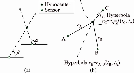
Fig. 1 Two kinds of seismic source location methods
There are a lot of researches on the influence factors of location accuracy. The sensors array or the seismic networks station, the sensitivity and precision of sensors, the difference of arrival time (TDOA), wave velocity model and the source location algorithm are the key factors which influence the accuracy of seismic source localization. Regarding the error from wave velocity model: In the 1970s, the suppression-subtractive hybridization (SSH) method is proposed by CROSSON [18], who makes speed as a variable in the source localization process, and calculates the source joint speed. It reduces the error to some extent because of the proposed speed model. But, the introduction of the unknown parameter will increase the amount of calculation and make the solving process not so stable. In 2008, LI and DONG [19,20] proposed a method without pre-measuring speed, significantly reduced the error result from velocity measurement. Also, they discussed the three-dimensional analytical solution of this problem [21,22]. In terms of the error due to microseism network, KIJKO [23,24] thought that microseism network has a significant effect on the source location accuracy, GONG et al [25] established genetic algorithm model for large-scale network planning problem by D value optimization theory; TANG et al [26] and JIA and LI [27] researched microseismic monitoring network optimal placement in deep metal mines and coal mines respectively [26,27]. LI [10] and GE [5,6] verified that with the increase of the distance between source and sensors, the location accuracy and stability are decreasing consistently and nonlinearly [10].
Considering the different importance of each sensor in location, the relocation method is proposed in this work. Here, the data of each sensor will be validated according to the probability and reliability of data, the erroneous data will be removed prior. And then the part of some optimal equation groups will be picked out by the procedure of equations selection. The final location is considered to be the average result from all selected high-confidential equation groups.
2 Problem and motivation
Firstly, the problem description and the terminology of this paper will be given out. The goal of source location is getting the location of a microseism by sensor data. Assuming that the location of the source is (x, y, z), it is an unknown variable, and it is the target of our research. t denotes the time when the microseism event generated. It is also unknown, but it can be gotten as long as the source location is known. The number of sensors is N, and the location of the ith sensor is (ai, bi, ci) (i=1, 2, ��, N), this is known beforehand. The time when the microseismic wave arrived the ith sensor is ti, which is known. And ti-tj, named time delay of arrival (TDOA for short), will be denoted as ��ij. The velocity of the waveform is v, which is a constant and can be measured beforehand. Then, the location of the source can be transform to a classical propagate problem in the homogeneous medium as follows.
 (1)
(1)
It can be transformed by subtracting two equations (1) with different sensors i and j introduced.
Di-Dj=v(ti-tj) (2)
The location of microseism can be gotten from above equations if the number of sensors is greater than 4 in 3-dimensional space, or the number is greater than 3 in 2-dementional space. There are a lot of researches about how to solve the Eq. (2), such as Refs. [10,14,20]. In these traditional methods, nearly all sensors data are used to construct equation with the same weight value. This will inevitably introduce errors in the following two steps, so we specifically put forward two strategies to optimize the calculation results according to these two steps respectively. 1) Inappropriate data or failed sensors may bring in error. Some random factors may cause some abnormal data of sensors, for example, instability of circuit, field construction, system error or some human influence. These abnormal data would introduce considerable errors to the ultimate location. Therefore, they should be picked out and discarded before computing. 2) Inappropriate equations may amplify the measurement error. In practice, it can often be found that the error of location varies considerably when different sensor data are used. Figure 2 gives an example, where solid line is the original hyperbola without errors, and the dashed line is the hyperbola with noise. In two subfigures of Fig. 2, TDOA is the same, but one of the hyperbola is different, and then the location error makes a significant difference. From the figure, we can found that the included angle of two hyperbolae in Fig. 2(a) is higher than that in Fig. 2(b).
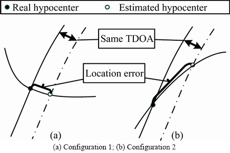
Fig. 2 Principle of sensors data effect on location precision
As Fig. 2 shows, if some inappropriate equation combinations are used in calculation, the sensor error will be amplified in the final location result. Therefore, we expect to choose the data with high reliability and the reasonable combination of equations with optimal noise tolerance to get the more accurate microseismic source location, in which, the data with high reliability could be selected according to the voting principle and propagation theory. In terms of the equation selection, is determined the approximate location of a micro source according to the traditional method, and equations with optimal noise tolerance are selected according to the relative position relationship between the source and sensors, then the exactly source location is gotten.
3 Model
Here we present a new method named relocation method to solve the select problem of the optimal sensors data and equation groups respectively.
3.1 Voting method and constraint method
3.1.1 Voting method
It is assumed that most of the sensor data are normal, while a little may be exceptional, i.e., with a high error. Then we can design a method which could identify those exceptional data by a voting mechanism and get a better location result. The voting method is described in Algorithm 1. Here, the location and TDOA of sensors are known. Then we will search all possible combination of four sensors (because four sensors are the minimum number of locating a source in 3-dimentional space) to get C(N, 4) different locations of the source, as step 1 shows. Then the k-mean method is used to find out a reliable centre of those possible locations of the source. Here, reliable centre means that most of the locations are close to this point. If a location fixed by sensor S1, S2, S3 and S4 belongs to the biggest cluster, then the credit of S1, S2, S3 and S4 will increase respectively. The outstanding 80% sensors with higher credit value will be kept for future computation.
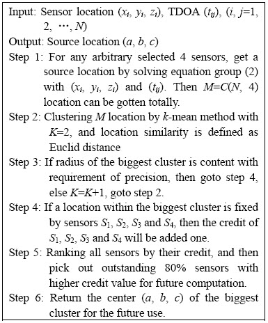
Algorithm 1 Voting method
3.1.2 Constraint method
Assuming S1 and S2 are two sensors, O is the microseismic source. According to the theory that the sum length of any two edges of a triangle is not less than the third one, it can be easily known:
 (3)
(3)
where S1S2 means the distance between two sensors.
If the velocity of the waveform is v, then we can get the following inequality from Eq. (3) directly.
 (4)
(4)
where S1S2, t1, t2, and v are all known. Therefore, we can get C(N, 2) constraint inequality totally. If the two sensors data did not meet the inequality, they would be removed. The procedure is described in Algorithm 2. In the algorithm, each pair of sensors data will be checked to see if they meet the inequality. If not, they will be deemed as untrustworthy data, and will be removed from the data set. The return value of algorithm is the reliable data set.
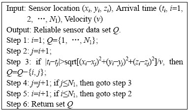
Algorithm 2 Constraint method
If constraint method is executed first, it is probable that data with larger error will make all other data to be discarded. Therefore, in the process of picking data, the voting method should be executed first, and then the constraint method is performed.
3.2 Combination of equations
At least four sensors are needed to compute a location in 3-dimentional space. Then we will discuss how the location error will be affected by the distribution of sensors. Assuming four sensors are S0(a0,b0,c0), S1(a1,b1,c1), S2(a2,b2,c2), S3(a3,b3,c3), respectively, then we can list the following equations.
Di=d(ai, bi, ci)=v(ti-t), i=0, 1, 2, 3 (5)
��Di=Di-D1=v(ti-t1), i=1, 2, 3 (6)
If we differentiate two sides of Eq. (6) at the same time, we can get Eq. (7).
d��Di=vd��i0=(Ci1-C01)dx+(Ci2-C02)dy+(Ci3-C03)dz, i=1, 2, 3 (7)
where
 (8)
(8)
Then we rewrite Eq. (7) to array forms as follows.
vd��0=K�� (10)
where
d��0=[d��10d��20d��30]T (11)
��=[dx dx dz]T (12)
 (13)
(13)
Pseudo-inverse method can be used to solve Eq. (10), then
 =v(KTK)-1KTd��0 (14)
From Eq. (14), mean value of the location error can be denoted as follows:
 (15)
(15)
Because the above equation is nonlinear, there is no obvious solution. Therefore, simulation is used to get the closest solution. For the sake of obtaining better performance sensors, we divide the layout of four sensors into the following categories and discuss their merits and drawbacks respectively.
Situation 1: S0S1S2S3 in the same plane. Here the arrangement that four sensors located at four corners of a square is simulated, the side length of the square is 10 km, d��0=[0.1 ms, 0.1 ms, 0.1 ms]. Figure 3 shows the mesh graph of E computed according to Eq. (15). By the simulation, it is found that singular area exists in plane S0S1S2S3. If the source is in this area, the error will be high. So if sensors distributed like this, they should not be considered to locate the source effectively.
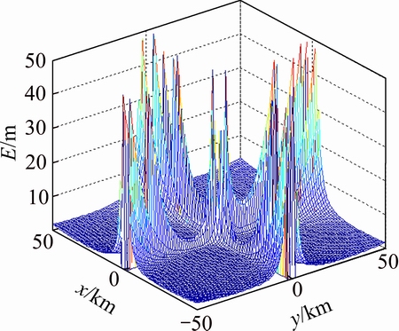
Fig. 3 Error distribution for situation 1
Situation 2: S0S1S2S3 are on the four corners of a tetrahedron respectively, and the projection of S0 to plane S1S2S3 locates outside of the triangle S1S2S3. Here, we assign sensors S1, S2 and S3 located at three corners of a square with side length of 10 km, and the projection of S0 to plane S1S2S3 locates to the rest corner. d��0=[0.1 ms, 0.1 ms, 0.1 ms]. Figure 4 shows the mesh graph of E computed according to Eq. (15). By the simulation, it is found that there exists singular area in and out the triangle S1S2S3. If the source is in this area, the error is colossal. So, it is not a good choice for locating the source accurately if sensors distribute like this.
Situation 3: S0S1S2S3 are on the four corners of a tetrahedron, and the projection of S0 to plane S1S2S3 locates on the edge of the triangle S1S2S3. Here, we assign sensors S1, S2 and S3 located at three corners of an equilateral triangle with side length 10 km, and the projection of S0 to plane S1S2S3 situated on the line of S1S2. d��0=[0.1 ms, 0.1 ms, 0.1 ms]. Figure 5 shows the mesh graph of E computed according to Eq. (15). By the simulation, it is found that there exists singular area in and out the triangle S1S2S3. If the source is in this area, the error is very significant. So, if sensors distribute like this, they should not be considered to locate the source effectively.
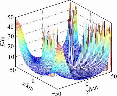
Fig. 4 Error distribution for situation 2
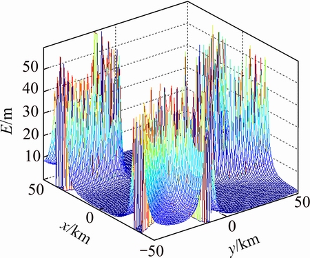
Fig. 5 Error distribution for situation 3
Situation 4: S0S1S2S3 are on the four corners of a tetrahedron, and the projection of S0 to plane S1S2S3 locates inside of the triangle S1S2S3. Here, we assign sensors S1, S2 and S3 located at three corners of an equilateral triangle with side length of 10 km, and the projection of S0 to plane S1S2S3 situated in the center of triangle S1S2S3. d��0=[0.1 ms, 0.1 ms, 0.1 ms]. Figure 6 shows the mesh graph of E computed according to Eq. (15). By the simulation, it is found that it is convergent when the source is located on the triangle S1S2S3. When the source is outside the triangle, the error is also acceptable. Therefore, four sensors distributed like this are the best choice for the precise location.
From the above analysis, it is evident that when the source is located in the tetrahedron S0S1S2S3, it has a better performance. Then, we can design the following relocation algorithm.
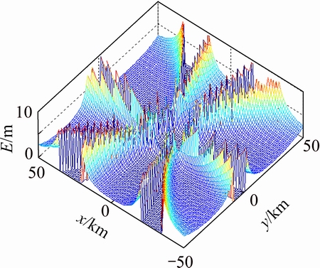
Fig. 6 Error distribution for situation 4
Algorithm 3 Process of relocation method
Here, the (a��, b��, c��) is gotten from algorithm 1, sensor location and TDOA are known. All sensor groups which include exactly four sensors (named S1, S2, S3, S4, respectively) are considered by algorithm 3 in step 2; if (a��, b��, c��) is located inside the tetrahedron S1S2S3S4, then we relocate the position of the source by these sensors and save the result as step 4. When all the sensor quaternaries are considered, the k-mean method is used to find out a precise centre of those possible locations of the source within all saved results and made it as the return value of the algorithm.
4 Experimental
The experiment has been divided into two parts. One is the simulation experiment, and the other is the field experiment. The traditional microseism source location method such as the global optimization method is selected as the reference. For the sake of brevity, we will name them RL(relocation method) and TL(traditional location method) in the ensuing paragraphs respectively.
4.1 Simulation
There are some complicated factors like system errors and noise level that cannot be controlled in real microseism application. Here, synthetized data are used to verify the relocation method. MATLAB is used to simulate a scene, and specify the distribution of the sensor position as shown in Fig. 7. Assume that the 10 km �� 5 km �� 2 km cubic is an ore body, in which 12 s are arranged at the corner and assigned to monitor the vibrated wave. Wave velocity is set as 5.0 km/s. And then 50 microseismic events are generated in space randomly and sequentially. The arrival time of seismic wave of sensor is calculated by the source location, sensors location and the assumed velocity.
In order to simulate the actual condition as much as possible, white noise is added to smear the simulated seismic wave. Then, these data are used to predict the source location by relocation algorithm and its counterpart. Four configures are assigned as Fig. 8 shows.
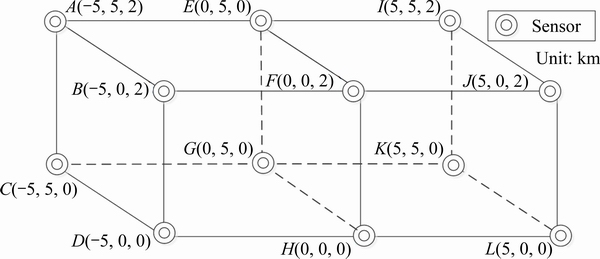
Fig. 7 Distribution of sensors
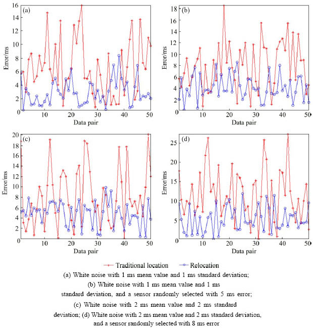
Fig. 8 Location errors when different TDOA are given (here N(��, ��) means a normal distribution with mean value �� and standard deviation ��)
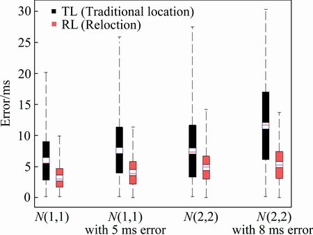
Fig. 9 Boxplot of location errors with different methods and TDOA errors
The experiment result is shown in Fig. 9, it can be found that when N (1 ms, 1 ms) normal TDOA errors is introduced, the location error of RL reduced by 36.5% compared with TL. When N (2 ms, 2 ms) is added to all TDOA, and 8 ms error is added to TDOA of a selected sensor pair, the location error of RL reduced by 39.1% than TL method. The result of other situations are shown in Fig. 9. It is obvious that RL method outperforms TL methods in each situation. It shows that the RL method has a better accuracy in simulation.
4.2 Field experiment
In order to prove the validity of the relocation method in reality, data from microseism monitor system of Dongguashan Copper Mine is chosen to verify the precision of the RL algorithm. The monitor system is called integrated seismic system (ISS), which is developed by South Africa ISS International Corporation. 18 single component sensors are arranged in three tunnels to monitoring microseismic events for 24 h for 365 d. Then, 3 blasting events with the known location are executed. The location coordinate of blast is shown in Table 1.
Table 1 Location of blast experiment
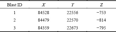
Table 2 Location of sensors
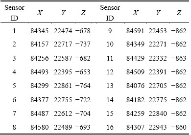
We take each blast as a microseismic event and predict the location of blasts by the arriving time recorded by sensors. There are 18 sensors deployed in the mine totally. The location of sensors is shown in Table 2.
Similar with the simulation part, the relocation method is compared with the traditional microseism source location method in field experiment. For each blasting event, the computation is executed 50 times with random TDOA error. And four noise levels are considered. The results are compared in Fig. 10. When N(1 ms, 1 ms) normal TDOA errors exist, the location error by RL method is reduced by 42.5% than TL method. When N(2 ms, 2 ms) normal TDOA errors and 8 ms assumed sensor error exist, the location error of RL method is reduced by 41.8% compared with TL method. The results of other situations are shown in Fig. 10. In general, the RL outperforms TL method and gives more accurate locating results in the field computation.
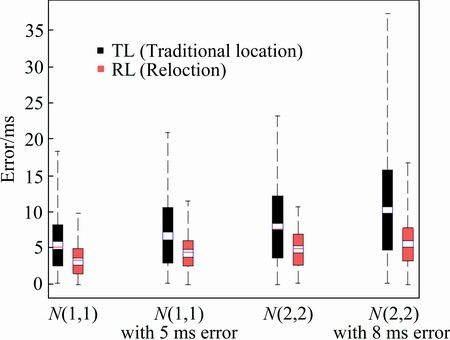
Fig. 10 Boxplot of location errors in field experiment
5 Conclusions
1) The location precision of micro-seismic source can be improved in following ways when there are abundant sensors data available: I) Removing incredible data by the constraint of the model; II) Removing the inappropriate equations that may amplify the sensor error; III) Voting for locations by different sensor groups by k-mean cluster.
2) The location error of relocation method is reduced by 41.8% compared with traditional location method when error of normal distribution with mean value 2 ms is added.
3) The relocation method can improve the fault-tolerant performance significantly and get more accurate location results. It will play an important role in later practical application. In future, we will explore the use of machine learning in removing both incredible data and inappropriate equations.
References
[1] ORTLEPP W D. RaSiM comes of age��A review of the contribution to the understanding and control of mine rockbursts [C]//Proceedings of the Sixth International Symposium on Rockburst and Seismicity in Mines. Perth, Western Australia, 2005: 9-11.
[2] Zhao G Y, Bing D A I, Dong L J, Chen Y A N G. Energy conversion of rocks in process of unloading confining pressure under different unloading paths [J]. Transactions of Nonferrous Metals Society of China, 2015, 25(5): 1626-1632.
[3] Dong L J, LI X B, PENG K. Prediction of rockburst classification using random forest [J]. Transactions of Nonferrous Metals Society of China, 2013, 23(2): 472-477.
[4] ZHAO G Y, MA J, DONG L J. Classification of mine blasts and microseismic events using starting-up features in seismograms [J]. Transactions of Nonferrous Metals Society of China, 2015, 25(10): 3410-3420.
[5] GE M. Analysis of source location algorithms: Part I. Overview and non-iterative methods [J]. Journal of Acoustic Emission, 2003, 21: 14-28.
[6] GE M. Analysis of source location algorithms: Part II. Iterative methods [J]. Journal of Acoustic Emission, 2003, 21: 29-31.
[7] Mohebi J, Zadeh SHIRAZI A, Tabatabaeec H. Adaptive- neuro fuzzy inference system (Anfis) model for prediction of blast-induced ground vibration [J]. Science International, 2015, 27(3): 2079-2091.
[8] Leighton F, Duvall W I. A least squares method for improving rock noise source location techniques [R]. Bureau of Mines, Washington, DC (USA), 1972.
[9] Zhao G Y, MA J, Dong L J, Li X B, Chen G H, Zhang C X. Classification of mine blasts and microseismic events using starting-up features in seismograms [J]. Transactions of Nonferrous Metals Society of China, 2015, 25(10): 3410-3420.
[10] LI Nan. Research on mechanisms of key factors and reliability for microseismic source location [D]. Xuzhou: China University of Mining and Technology, 2014. (in Chinese)
[11] Kang P, Wang Z, Sun J. Generation of artificial earthquakes for matching target response unsmooth spectrum via wavelet package transform [J]. Transactions of Nonferrous Metals Society of China, 2014, 24(8): 2612-2617.
[12] Sheen D H. A robust maximum-likelihood earthquake location method for early warning [J]. Bulletin of the Seismological Society of America, 2015, 105(3): 1301-1313.
[13] Engdahl E R. Advances in global seismic event location [C]//Advances in Seismic Event Location. Netherlands: Springer, 2000: 3-22.
[14] Thurber C H. Nonlinear earthquake location: Theory and examples [J]. Bulletin of the Seismological Society of America, 1985, 75(3): 779-790.
[15] Douglas A. Joint epicenter determination [J]. Nature, 1967, 215: 47-48.
[16] Menke W. Geophysical data analysis: discrete inverse theory [M]. Pittsburgh: Academic Press, 2012.
[17] Li N, Wang E, Ge M, Sun Z. A nonlinear microseismic source location method based on simplex method and its residual analysis [J]. Arabian Journal of Geosciences, 2014, 7(11): 4477-4486.
[18] Crosson R S. Crustal structure modeling of earthquake data: 1. Simultaneous least squares estimation of hypocenter and velocity parameters [J]. Journal of Geophysical Research, 1976, 81(17): 3036-3046.
[19] DONG L J, LI X B, TANG L Z, GONG F Q. Mathematical functions and parameters for microseismic source location without pre-measuring speed [J]. Chinese Journal of Rock Mechanics and Engineering, 2011, 30(10): 2057-2067.
[20] Dong L J, LI X B. A microseismic/acoustic emission source location method using arrival times of PS waves for unknown velocity system [J]. International Journal of Distributed Sensor Networks, 2013, 9(10): 307489.
[21] Dong L J, LI X B, ZHOU Z. Three-dimensional analytical solution of acoustic emission source location for cuboid monitoring network without pre-measured wave velocity [J]. Transactions of Nonferrous Metals Society of China, 2015, 25(1): 293-302.
[22] Dong L J, LI X B. Three-dimensional analytical solution of acoustic emission or microseismic source location under cube monitoring network [J]. Transactions of Nonferrous Metals Society of China, 2012, 22(12): 3087-3094.
[23] Kijko A. An algorithm for the optimum distribution of a regional seismic network [J]. Pure and Applied Geophysics, 1977, 115(4): 999-1009.
[24] Kijko A. An algorithm for the optimum distribution of a regional seismic network-2: An analysis of the accuracy of location of local earthquakes depending on the number of seismic stations [J]. Pure and Applied Geophysics, 1977, 115(4): 1011-1021.
[25] Gong S Y, Dou L M, Ma X P, Mu Z L, Lu C P. Optimization algorithm of network configuration for improving location accuracy of microseism in coal mine [J]. Chinese Journal of Rock Mechanics and Engineering, 2012, 32(1): 7-17.
[26] Tang L Z, Yang C X, Pan C L. Optimization of microseismic monitoring network for large-scale deep well mining [J]. Chinese, Journal of Rock Mechanics and Engineering, 2006, 25(10): 2036-2042.
[27] Jia B X, Li G Z. The research and application for spatial distribution of mines seismic monitoring stations [J]. Journal of China Coal Society, 2010, 35 (12): 2045-2048. (in Chinese).
һ���������Դ�Ķ��ζ�λ����
�����1,2����Ϧ��1����¤��1���ų���3��������1
1. ���ϴ�ѧ ��Դ�밲ȫ����ѧԺ����ɳ 410083��
2. School of Civil and Mechanical Engineering, Curtin University, Perth 6102
3. �ϻ���ѧ ����Դ����ѧԺ������ 421000
ժ Ҫ���������������һ���µĶ��ζ�λ�ķ����������״�ϵͳ�����ô����Ĵ�������Ϣ�����ʹ��������������Զ�λ��ɵ�Ӱ�죬����ͨ����������֮�佻���������߶�λ�ľ��ȡ������Ĺ����ǣ����ȸ��ݴ�����λ�õ����ظ���ÿ���������������ݵĿɿ��ȣ�ʹ�ÿɿ��Ƚϸߵ����ݽ�����Դλ�õij������㣬Ȼ����ݳ�ʼ��λ�Ľ���ʹ�����λ�õ���Թ�ϵѡ����������������̶ȵ�һ�鷽�̣���ͨ��k-meanͶƱ��ȷ�����յ���Դλ�á��Դ�ͳ��λ�����ͱ���������������˱Ƚ�����֤�����Ŀɿ��ԣ����ֱ�ʹ��ģ����ֳ��������ݽ����˶�λ���㡣���ֳ������У���TDOA������N(2,2)����̬�ֲ����봫ͳ������ȣ����ķ����Ķ�λ������41.8%��ʵ����������������Ķ��ζ�λ���ܹ���������ݴ����ܣ��õ���Ϊ��ȷ�Ķ�λ�����
�ؼ��ʣ��𣻶��ζ�λ��k-mean������ѡ����������
(Edited by Yun-bin HE)
Foundation item: Projects (11472311, 41272304, 51504288) supported by the National Natural Science Foundation of China
Corresponding author: Xi-bing LI; Tel: +86-731-88877254; E-mail: xbli@csu.edu.cn
DOI: 10.1016/S1003-6326(16)64429-1
Abstract: A new method, named relocation, was proposed to reduce the impact of sensor errors systematically, especially when available data of sensors are abundant. The procedure includes evaluating the reliability of every sensors datum, processing the initial location by the credible data, and selecting a set of equations with optimal noise tolerance according to the relative relationship between the initial location and sensors location, then calculating the final location by k-mean voting. The results obtained in this research include comparing traditional location method with the presented method in both simulation and field experiment. In the field experiment, the location error of relocation method reduced 41.8% compared with traditional location method. The results suggested that relocation method can improve the fault-tolerant performance significantly.
