

J. Cent. South Univ. (2019) 26: 743-758
DOI: https://doi.org/10.1007/s11771-019-4044-4

A new approach for on-line open-circuit fault diagnosis of inverters based on current trajectory
LI Kai-di(���)1, CHEN Chun-yang(�´���)1, CHEN Te-fang(���ط�)1,CHENG Shu(����)1, WU Xun(�髑)2, XIANG Chao-qun(��Ⱥ)1
1. School of Traffic and Transportation Engineering, Central South University, Changsha 410075, China;
2. School of Automation, Central South University, Changsha 410083, China
 Central South University Press and Springer-Verlag GmbH Germany, part of Springer Nature 2019
Abstract:
Security and reliability of inverter are an indispensable part in power electronic system. Faults of inverter are usually caused by switch elements�� operating fault. Taking the inverter with hysteresis current control as the research object, a universal open-circuit fault location method which can be applied to multiple control strategies is proposed in the paper. If the switch open-circuit fault happens in inverter, the output phase current will inevitably change, which can be used as a characteristic for diagnosis, combined with the comparison of phase-current direction before and after the fault occurrence, to diagnose and locate the open-circuit fault in a half cycle. Moreover, this method requires neither system control signals nor sensor. The validity, reliability and limitation of the fault location method in the paper are verified and analyzed through dSPACE-based experiment platform.
Key words:
fault diagnosis; hysteresis; inverter; fault location��
Cite this article as:
LI Kai-di, CHEN Chun-yang, CHEN Te-fang, CHENG Shu, WU Xun, XIANG Chao-qun. A new approach for on-line open-circuit fault diagnosis of inverters based on current trajectory [J]. Journal of Central South University, 2019, 26(3): 743�C758.
DOI:https://dx.doi.org/https://doi.org/10.1007/s11771-019-4044-41 Introduction
Power electronics system has always been an important part of industrial production, and its safety and stability have become two important indicators for evaluating power electronic system. In general, the faults of power electronic system start from the part components, such as motor, inverter and sensor [1]. According to the statistical data, the proportion and severity of inverter faults are listed in the forefront of power electronic system [2�C4]. Generally, the inverter failures are caused by the capacitor failure, the semiconductor switch failure, and the drive circuit failure, and so on [5]. The semiconductor switches are the most fragile and vital part, but its faults proportion is 21% in the whole system faults [2, 4]. Therefore, the technologies about how to realize semiconductor-switch fault diagnosis are becoming a research hotspot in recent years. And insulated gate bipolar transistor (IGBT) switch device is the most widely applied in semiconductor switches. The current diagnostic methods can be classified into different kinds by their diagnostic ideas.
The first kind is the methods based on intelligent algorithm [7�C11]. The work in Ref. [7] proposes a machine-learning fault diagnostic method for induction motor drives by the structured neural network. Most usual kinds of failures including single switch open-circuit failure, post short-circuits failure, and the unknown failures can be detected and isolated through this method. In Ref. [8], the open circuit fault of inverter is diagnosed and located by using wavelet transform to extract diagnostic indices, then using radial basis function neural network to identify diagnostic data, and finally diagnosis the fault through the data. By the feature analysis for the output currents of different states, a fault diagnostic method is proposed in Ref. [9], which by using multistate data processing block and subsection fluctuation analysis block processes data and the artificial neural network block to implement intelligent classification. The work in Ref. [10] proposes a Bayesian-networks-based data-driven algorithm. The process knowledge and training data are needed for diagnosis, which is not applicable in some of the actual diagnosis. In Ref. [11], a fault diagnosis method based on Bayesian networks is proposed. It collects the line voltage on the output side of different fault models and extracts the fault characteristics, then carries out fast Fourier transform, finally makes fault diagnosis via Bayesian network. The fault diagnosis methods of this category require a great deal of calculation, and the uncertainty of the neural network structure will lead to the error in the judgment of some intermediate link, thus affecting diagnosis accuracy. Moreover, this kind of method applications is largely limited by data samples.
The second kind is model-based fault diagnosis [12�C15]. By analysis and comparison of the switch function models of the inverter under normal and fault state, a fast fault diagnosis method without sensors is proposed [12]. ALAVI et al [13] proposes a model-based diagnosis method for multi-level multi-phase voltage source inverters (VSI). The fault can be detected by monitoring pole voltage of each phase, then certain switching modes are applied to locating the fault. In Ref. [14], an on-line model-based diagnosis method for half-bridge inverter is proposed. The hybrid bond graph model of the circuit is established and the pattern recognition technology is applied to calculating switch status, so the inverter short-circuit fault can be diagnosed. By using Baum-Welch algorithm for iterative training and Viterbi algorithm for fault identification, a fault diagnosis method based on hidden Markov model is proposed [15]. The fault diagnosis methods of this category are based on accurate model, they diagnose the fault by using the characteristic parameters of the model. However, these methods usually require system control signals as model input, which are usually difficult to obtain or measure, and the calculation steps of them are complicated. Moreover, their applications are limited by fault model accuracy.
In the third kind, the existing diagnostic methods are based on signal processing [16�C24]. Most of category methods are voltage-based methods or current-based methods. The output voltage or current signals have been used for open-circuit and short-circuit faults for diagnostic objectives all the time. A fault diagnosis technology based on output voltage is proposed [16], which compares the preprocessed diagnosis eigenvalue and the voltage envelope. So single power module open-circuit fault can be detected by this technology. But this method is not applicable for hysteresis current control strategy. The fault diagnosis method for inverter proposed in Ref. [17] is based on the deviation of the normalized actual pole voltages of every bridge arm and the corresponding reference bridge-arm status. Therefore, the implementation requires the measurement of every bridge-arm status. This method has a wide range of applications but requires additional sensors. WU et al [18] proposes a voltage-based fault diagnosis method which aims at voltage source converters. The method is achieved by obtaining the reference voltages of the system control signal. Thus, this method does not need extra sensor, but the system control signal is necessary and the algorithm is much complicated. Refs. [16�C18] are all voltage-based methods, although they have some inherent advantages, they usually require additional sensors, or their diagnosis algorithms are relatively complex. On the other hand, current-based methods can avoid obtaining system information and they do not need extra sensor. HE et al [19] proposes a current trajectory based method. The trajectory is a graph which is complying with standard elliptic equation in the Cartesian coordination under normal condition. If the fault happens, the graph becomes distorted and the fault will be located by the graphic parameters of the graph. Although it is able to locate double switch open-circuit faults, the algorithm is a bit complex. Besides, the performance under space vector pulse width modulation (SVPWM) control strategy and hysteresis current control strategy are not evaluated. YAN [20] proposes a current-based diagnosis method, which collects the unusual changes of the direct-current-bus neutral-point current signals, then integrates with the previous data of transient switch status and phase currents to achieve fault diagnosis. Based on the phase current reconfiguration technology, JLASSI et al [21] proposes an open-circuit failure location method for the low-power VSI. But Refs. [20, 21] require additional sensors. In Ref. [22], a method which can diagnose multiple open-circuit faults is proposed; the phase current is processed to have no connection with the operating status, then this phase-current signal can be adopted as the diagnostic feature. However, the computation is huge, the diagnostic accuracy and the time consumption are related to the value of empiric threshold. Based on output current online identification, an adaptive technique of condition monitoring is proposed [23]. However, the accuracy of the algorithm still needs to be improved. In Ref. [24], a method is proposed for three level inverters and can diagnose both the single switch fault and diode fault, but the algorithm in this paper is too complex.
In general, the huge short-circuit current will inevitably cause the breakdown of the working system. Thus, the short-circuit faults are usually well-prevented to guarantee the safety of whole system [25]. And the short-circuit faults are usually transformed into the open-circuit fault by fuse protection [26]. Therefore, this paper majorly studies the open-circuit fault of inverter. The proposed open-circuit fault diagnostic method is based on output-side phase current trajectory. The faults are judged and located by the contrast of the output-side phase current trajectory under normal condition and fault condition. And this method requires neither system control signals nor sensor. The single switch fault can be detected in half phase-current period faster than the reported methods. Moreover, the method proposed in this paper has good reliability, and the diagnosis accuracy is independent of load change. This diagnostic method not only can be applied in the inverter with hysteresis current control strategy, but also sinusoidal pulse width modulation (SPWM) control strategy, and SVPWM control strategy, the output-side phase current of which has periodic variation. Furthermore, as the frequency increases, the time of diagnosis will decrease.
The rest of the paper are arranged as follows: Section 2 analyses the three-phase bridge inverter circuit and the mechanism of open-circuit fault, Section 3 proposes a novel switch open-circuit fault location technology, Section 4 presents a dSPACE-based fast diagnosis platform and validates the method proposed in this paper by experimental data, and Section 5 makes the summary of this paper.
2 Analytical model
In this section, we first introduce the model of hysteresis current control inverter, then propose an analytical model for inverter open-circuit fault.
2.1 Hysteresis current inverter model
Hysteresis current control is a closed-loop control technique, which uses the deviation of instruction current and actual output current as the input of hysteresis comparator to control the switching of power device that directly leads to rise and fall of the output current, resulting in an obedience of the output current to the instruction current trajectory. Figure 1 shows a typical topology of three-phase bridge inverter circuit with hysteresis current control. Ud denotes the DC voltage, i* represents the instruction current, and i is the actual phase current. V1�CV6 are the power devices and VD1�CVD6 are the diodes. LA, LB, LC and RA, RB, RC are the resistance-inductance loads. Since the three single-phase branches are isomorphic, we can take an arbitrary branch, e.g., phase-A circuit in Figure 1, to demonstrate the principle of hysteresis current control without loss of generality, as presented in Figure 2. The phase current in a single-phase branch is shown in Figure 3.
In Figure 2, ifb is the feedback current on the output side, h is the bidirectional band range of the hysteresis comparator, RA and LA are the resistance and inductance on the load side, respectively, uo is output-side AC voltage (its value is Ud) and io is the output-side AC current. Therefore, the load-side differential equation is shown below:
 (1)
(1)
Both the starting conditions which can reveal the operating status of energy storage element and formula (1) combine to deduce the transient process of output-side phase current. According to the control features of hysteresis current strategy, the transient process of output-side phase current can be divided as the following four categories.
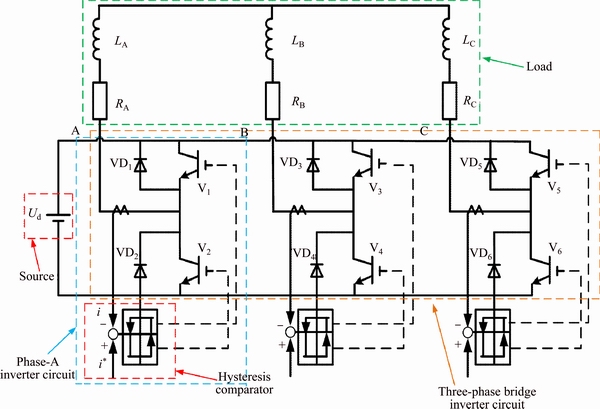
Figure 1 Three-phase bridge inverter circuit with hysteresis current control
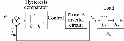
Figure 2 Simplified diagram of phase-A circuit with hysteresis current control
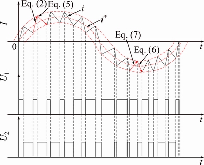
Figure 3 Current trajectory of hysteresis current control circuit
If the output-side phase current is in the interval io>0 and the value of io is less than or equal to the band range of the instruction current, the comparator gives the [ON] signal to switch V1, so the output-side phase current is increased. The operating status of V1 is [ON], that is, uo=Ud, the solution of Formula (1) is given as follows:

or
 (2)
(2)
In Formula (2), ��=L/R is inertia time constant. Ifbm=Ud/R is the steady-state maximum of the feedback current ifb. The corresponding transient current trajectory of phase current is given in Figure 3, which can be denoted with Formula (2).
If the output-side phase current is in the interval io>0 and the value of io is larger than or equal to the band range of the instruction current, the comparator gives the [ON] signal to switch V2, so the output-side phase current is decreased. In this condition, the operating status of fly-wheel diode VD2 is [ON]. Because of the existence of inductance L, the phase current can not change abruptly (In order to simplify the control logic, the control signals of V2 and V1 are complementary. However, no current will pass through because of its unidirectional conduction characteristic). In this situation, the circuit can be regarded as a zero-input response circuit, as shown in Figure 4. In the figure, iL(t) is the inductive current, UR(t) is the voltage drop across the resistor, and UL(t) is the inductive voltage.
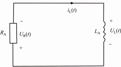
Figure 4 Equivalent circuit diagram of fly-wheel diode [ON]
It is set the inductive current iL(t) before the switch changes to be iL(0+)=Io+. The differential equation of the circuit is given according to the Kirchhoff��s law:
 (3)
(3)
The solution of Formula (3) is:
 (4)
(4)
In Formula (4), D denotes integration constant which is decided by the starting conditions. Thus
 (5)
(5)
Figure 3 shows the transient current trajectory of phase current, which can be denoted with Formula (5).
If the output-side phase current is in the interval io<0 and the value of io is larger than or equal to the band range of the instruction current, then V2 is controlled to decrease the phase current. The operating status of V2 is [ON], the analysis process is the same as switch V1. In this situation, uo=�CUd, so the solution of Formula (2) is given:

or
 (6)
(6)
Figure 3 shows the transient current trajectory of phase current, which can be denoted with Formula (6).
Similarly, if the output-side phase current is in the interval which io<0 and the value of io is less than or equal to the band range of the instruction current, then V1 is controlled to raise the phase current. The operating status of V2 is [ON]. The analysis process is the same as fly-wheel diode VD2. It is set the inductive current iL(t) before the switch changes to be iL(0�C)=Io�C. (At this stage, V1 is the same as the V2 above), thus:
 (7)
(7)
Figure 3 shows the transient current trajectory of phase current, which can be denoted with Formula (7).
2.2 Mathematical model for faulty inverter
When the inverter occurs the IGBT open circuit faults, in the case of an upper-tube fault (such as phase-A V1), the fault will degrade performance of the feedback loop in tracking instruction current when i*>0. If the fault occurs when the actual phase current i>0, the current i is unable to change abruptly due to the effect of the inductor L. So i will descent from the current value to zero. The descent speed is determined by the value of inductance L, and the specific descent process corresponds to Formula (5). The tracking will not start till the instruction current i*<0. In the other case, if the fault occurs when the output phase current i<0, it tracks the instruction current when i*<0 until i*��0. Then, i remains zero during the period when the instruction current i* >0. Until the instruction current comes to the interval i*<0, the tracking resumes. In the case of a lower-tube fault (such as phase-A V2), the performance of the feedback loop in tracking instruction current i*<0 is degraded. The analysis procedures are similar to the case of positive interval, and the result is the opposite.
Consequently, the analytical models of single-phase current hysteresis control circuit��s upper and lower tube fault can be derived respectively.
Upper tube fault:
 (8)
(8)
where is positive maximum and
 is negative maximum of the instruction current i*.
Lower tube fault:
 (9)
(9)
According to the above model, when an IGBT fault occurs in an inverter circuit, the phase current waveform will absolutely change. Based on this phenomenon, in this paper, the phase-A current is taken as an example, V1 faults (upper tube fault) and V2 faults (lower tube failure) are discussed respectively, which are classified into four categories:
2.2.1 V1 open circuit fault happens when i*>0
When the fault has just occurred in V1  the equivalent circuit diagram is shown in Figure 5(a). At this moment, only VD2 is in the fly-wheeling state, and the output current io will decrease from the initial value Io+ to 0. The shape of the decreasing current curve is related to the load. According to the mathematical model,
  when the instruction current satisfies
  the equivalent circuit is shown in Figure 5(b). In this case, V2 and VD1 are both in normal working state, and the output current io is normally tracking the instruction current i*, so that the output current io can be expressed by Formulae (6) and (7). When the instruction current returns to be positive in the next cycle
  the equivalent circuit diagram is shown in Figure 5(c). Since the upper and lower tubes of the phase-A circuit are in the state [OFF],the phase-A instruction current cannot be traced, such that the output current io(t)=0.
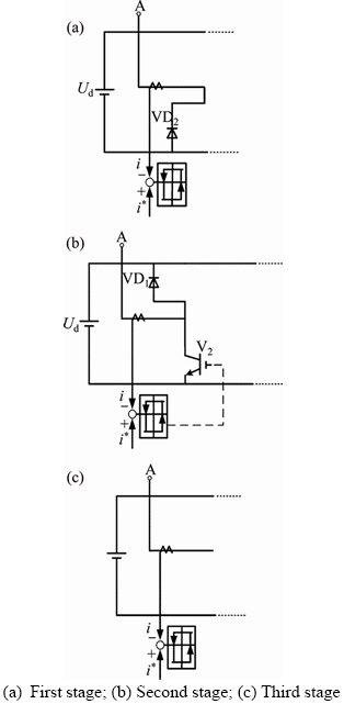
Figure 5 Fault equivalent circuit of case (1):
Therefore, the mathematical model of phase-A current under case (1) can be expressed as follow:
 (10)
(10)
Through Matlab/Simulink, under case (1), the inverter circuit phase-A current simulation waveform can be acquired, as shown in Figure 6.
We set the fault start time of case (1) as 0.204 s and the fault occurrence point is indicated by the red circle. In the first cycle of the fault, the output current io will decrease from the instantaneous value Io+ to 0, and remains at 0 during the period while the instruction current i* is still positive. Then the output current starts normally tracking the instruction current until the next cycle begins, and the output current remains at 0 during the period when the instruction current is positive. It has been circulating according to this rule since then. Because the fault of upper tube affects the performance of tracking the instruction current when i*>0, the specific location of the fault can be determined according to whether tracking direction is positive or negative. As shown in Figure 6, due to the loss of tracking function when the instruction current satisfies  the fact that upper tube occurs fault has been confirmed. It can be seen from Figure 6 that phase-A current trajectory is the same as the theoretical analysis and deduction process under the fault of case (1) condition.
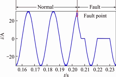
Figure 6 Fault output current waveform of case (1)
2.2.2 V1 open circuit fault happens when i*<0
The fault analysis of case (2) is similar to case (1), and it can be regarded as the special case of case (1) which skips the first fault cycle. The equivalent circuits of the two stages of case (2) are respectively shown in Figures 7(a) and (b). The mathematical model of the phase-A current of case (2) is expressed as:
 (11)
(11)
The phase-A output current simulation waveform under case (2) condition is shown in Figure 8.
2.2.3 V2 open circuit fault happens when i*<0
The fault analysis of case (3) is similar to case (1), while the directions of current and results are opposite. The equivalent circuits of the three stages of case (3) are respectively shown in Figures 9(a)�C (c). The phase-A current mathematical model in case (3) fault condition is as follows:
 (12)
(12)
We can also obtain the inverter circuit phase-A current waveform under case (3) condition by Simulink simulation.
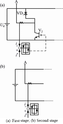
Figure 7 Fault equivalent circuit of case (2):
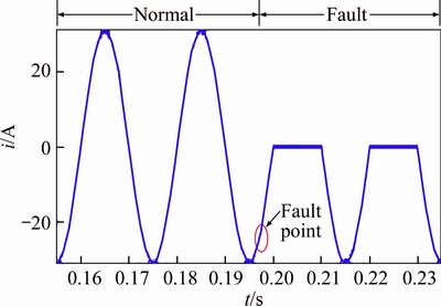
Figure 8 Fault output current waveform of case (2)
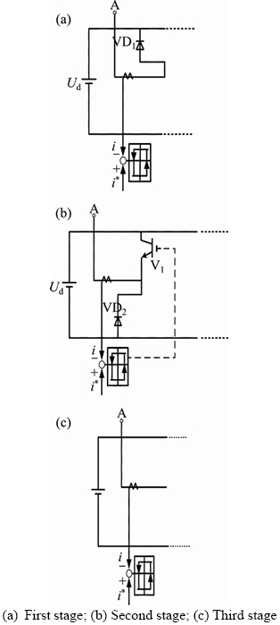
Figure 9 Fault equivalent circuit of case (3):
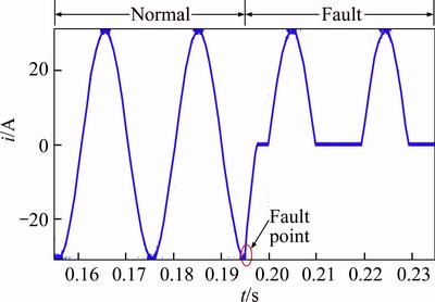
Figure 10 Fault output current waveform of case (3)
2.2.4 V2 open circuit fault happens when i*>0
The fault analysis of case (4) is similar to case (2), while the directions of current and results are opposite. The equivalent circuits of the three stages of case (4) are respectively shown in Figures 11(a) and (b). The phase-A current mathematical model in case (4) fault condition is as follows:
 (13)
(13)
The inverter circuit phase-A current simulation waveform under case (4) condition is as follows.
According to the above analyses, it can be found that the phase-A current waveform experiences distortion when the fault occurs in the inverter circuit with hysteresis current control. The most discernable sign of fault is in the time frame when io(t)=0. This sign can be used to diagnose the fault phase accurately and quickly, and the fault alarm can be sent to guarantee the safety of the system operation. Moreover, the analytical model and simulation can clearly distinguish the differences of the fault current waveform between the upper and lower tube, the differences are mainly in the direction of tracking instruction current. Therefore, we can locate the position of the fault according to the value of the current in the quarter cycle before the occurrence of the fault. Specific extraction methods and test settings will be described and analyzed in detail in the following sections.
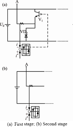
Figure 11 Fault equivalent circuit of case (4):
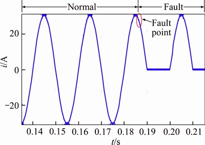
Figure 12 Fault output current waveform of case (4)
3 Fault location principle
3.1 Test setting
The topology of the three-phase bridge inverter circuit researched in the paper is shown in Figure 13.
In Figure 13, V1�CV6 are IGBTs with corresponding freewheeling diodes VD1�CVD6. DC-link components consist of R11�CR14 and C11�CC14, which are used for input voltage stablization. KM2 and R10 are used to prevent the current peak during the pre-charge stage. KM3 and R15 are discharge circuit, which releases the electricity after the inverter stops working. L1 is input reactor. Output filter components are composed of Laf, Lbf, Lcf and Caf, Cbf, Ccf. Ca�CCc are inductance-free capacitors.
In each phase of the circuit, two switches which are in series with IGBT are added to simulate the open circuit fault, such that each IGBT open circuit fault state can be simulated independently. The proposed fault detection method is simple as it does not require a large amount of devices and sensors added in the model. To locate the fault, it just needs to detect any two-phase current (such as iA and iB), and calculate the third phase current iC to monitor the fault status on-line. Moreover, when a fault occurs, the fault can be located accurately and an alarm will be sent within half of the cycle.
3.2 Fault characteristics extraction
According to the analytical model and the theoretical analysis, it should be noted that when the open-circuit fault occurs, there will be a special interval in which io(t)=0 holds for a certain time, by which the fault phase can be determined. Moreover, the waveforms of IGBT faults occurring at different times in different positions will also have their own unique characteristics in tracking directions. These two characteristics are considered to locate the specific location of inverter open circuit fault. Taking case (1) fault as the research example, the detailed analysis steps will be carried out below.
Based on the model of three-phase bridge inverter circuit under hysteresis current control, we can simulate the case (1) fault (upper tube fault, the fault happens, when i*>0). The open circuit fault start time of V1 is set as t1 (0.204 s), and the phase-A current waveform and the fault characteristic extraction diagram are shown in Figure 14.
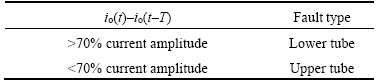
It is evident from Figure 14 that the distortion of the phase-A current waveform happens on t1, and after that point the phase current no longer tracks the instruction current as usual. In this paper, the extraction of fault characteristics is based on the special interval of io(t)=0. It can be observed that the disturbance of the current signal collected in the equipment usually results in a 2%�C3% fluctuation of the output current amplitude. For this interval, the threshold value is set as io(t)<1.5 (5% of the output current amplitude, as shown in Table 1, Ithr1 is the upper limit of the threshold, and Ithr2 is the lower limit of the threshold). There are 9 detection points in the model, the detection time span is 0.0002 s (1% of the length of a cycle). If all 9 detection points have detected io(t)<1.5, diagnosis system outputs high level signals. By this setting, it is possible to avoid erroneous judgment. When the output current drops to zero after the fault occurs and it maintains a certain period of time, then a fault alarm is sent (at t2 in Figure 14). In order to distinguish among phases, numerical amplification is applied to each phase. In diagnosis system, output 1 indicates the phase-A fault (system settings, output 2 indicates phase-B fault and the output 3 indicates phase-C fault), and output 0 indicates normal condition. Since the phase-alarm judgment is based on the output current waveform of each phase and each phase alarm system is independent of the others, the phase of open circuit fault can be located by phase current trajectory. Then, the waveform of the next fault cycle is used to determine the direction of the current loss ability of tracking instruction current. Finally, the diagnosis system sends out the fault location alarm (at t3 in Figure 14). The location of the fault tube can be quickly determined only by determining the direction. Thus, a module which subtracts itself is set up in the model and the module is set to delay one cycle. That is, the output waveform is subtracted from its own waveform of one cycle before, if the value is negative, then output 1, and conversely, output 2. Among them, output 1 indicates the upper tube, and output 2 indicates the lower tube. Considering the false alarm, the alarm threshold is set at 70% of the output waveform amplitude. As we can see from Table 2 (where T is a cycle) and Figure 15, in case (a), the fault occurrence time is t1 (0.204 s), and the alarming and phase location time is t2 (0.208 s), this process only takes 0.004 s (1/5 T). The case (a) fault in the first fault cycle is difficult to accurately determine the direction of lost tracking, which can be accurately judged in the second fault cycle at t3 (0.223 s), the consumed time is 0.019 s (about a cycle).
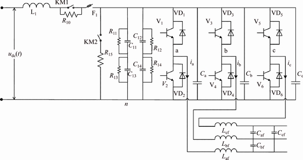
Figure 13 Diagram of three-phase bridge inverter circuit
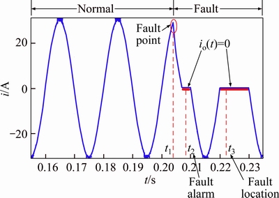
Figure 14 Phase-A current waveform and fault characteristic extraction diagram of case (a)
Table 1 Identification of open-circuit fault in phase-A
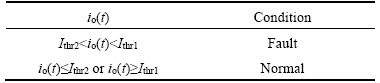
Table 2 Location of open-circuit fault in phase-A
4 Experiment
4.1 Experimental set up
The validity and reliability of the proposed diagnostic method are verified by a dSPACE experiment platform. Figure 15 gives an overview of the experimental system. The system mainly contains the inverter, load, and the dSPACE DS1007 PPC Processor Board. The control signals are created in dSPACE, then the signals are sent to the inverter through the input-output interface. The sensor signals are acquired from dSPACE through analog-digital conversion interface. Each phase current is monitored by the diagnostic module, and these monitoring data are sent to the computer for processing. The switches V1 and V2 open-circuit faults are taken as examples to verify the diagnostic method proposed in this paper.
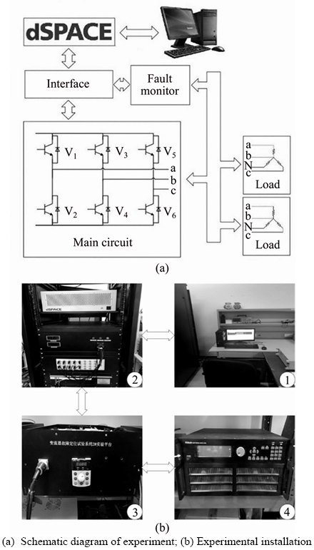
Figure 15 Experiment setting diagram:
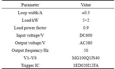
Table 3 Key parameters of experiment
4.2 Experimental result analysis
The cases (1), (2), (3), (4) types of open circuit faults are set at V1 and V2, respectively, and the fault location method is verified. The diagnosis waveform is shown in Figure 16, and the diagnosis results are shown in Table 4. In the experiment, the phase currents A and B are collected and monitored. After the open circuit fault happens, the fault is diagnosed and located according to the two obvious fault characteristics of phase current. Take case (1) fault as an example (Figure 16 (a)), it can be observed, the fault occurred at 0.205 s, after less than half cycle, the location of fault phase can be determined, and less than one cycle, the location of the fault tube can be determined. So the whole diagnosis process can be completed within one cycle. In the experiment, each phase tube has its own independent diagnosis and unique fault characteristics. In order to prevent the occurrence of misdiagnosis and false alarm, the thresholds are set up for the extraction and judgment of fault characteristics. Finally, according to the comparison between each phase output high level and Table 4, the location of the faulty tube can be diagnosed.
4.3 Reliability analysis
Due to the particularity of the current hysteresis control, the switching frequency of the inverter based on current hysteresis control is not a fixed value at a certain loop width. It will fluctuate within a certain range. The smaller the loop width is, the higher the frequency will be; the greater the loop width is, the lower the frequency will be. As shown in Figures 17(a) and (b) below, the loop width of fault characteristic extraction diagram is set as 0.5 A and 1.0 A, respectively. As we can see, when the loop width increases, the phase current waveform accuracy decreases, the tracking ability becomes weaker, and an obvious zigzag waveform appears, these are the phenomenon of the switching frequency drop. However, the fault characteristics extraction in this paper is based on io(t)=0 and two obvious characteristics of the direction of lost tracking. The change of loop width has little influence on it. It still can realize the function of fault phase alarming and fault tube location, so the method is adaptable to the change of loop width.
Load change is a common situation in practical applications. Two groups of experiments were set up to verify the adaptability of the diagnosis method to load change. The first group is set to cut off a set of load at 0.168 s (the original two sets of identical loads work together). The fault characteristic extraction diagram at this point is shown in Figure 18(a). Because the current hysteresis control target is current, if the current changes in the range where the inductance is able to withstand when the loads change, it is still able to achieve the tracking function. Therefore, the waveform is not changed greatly, and the location of the fault will not be affected. The second group sets the cut off at 0.168 s, as shown in Figure 18(b). At this point, the instruction current is raised, so that the output current is changed to track the instruction current after the load cut off, and thus the output current value has changed. However, the fault characteristic value of the diagnostic method is independent of the current amplitude change, so it will not affect the fault alarm and the location of the fault tube. It can be seen that the diagnostic method is independent of the load change.
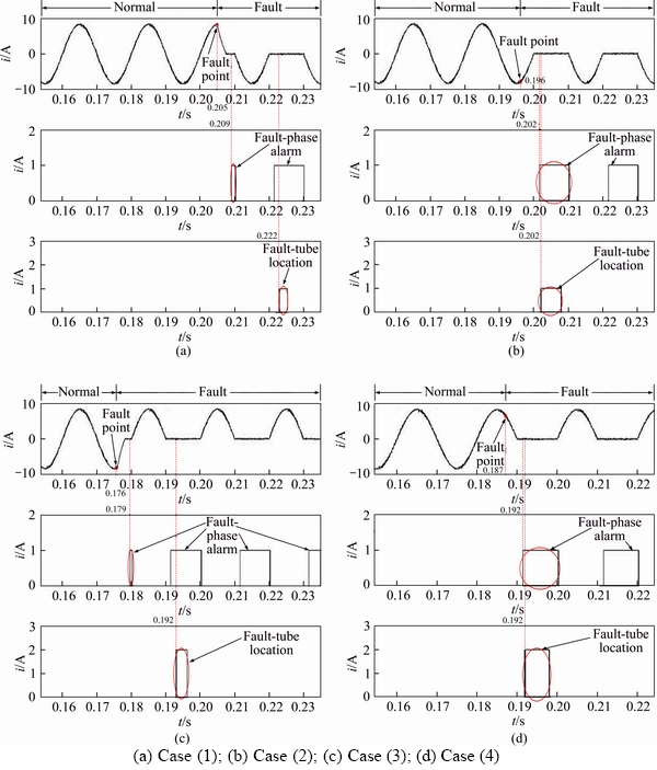
Figure 16 Open circuit fault output current waveform and fault diagnosis diagram:
Table 4 Fault location code table
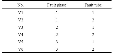
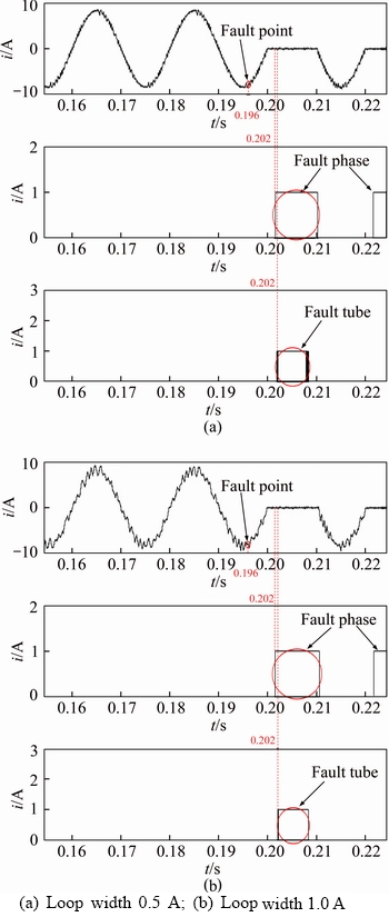
Figure 17 Experimental current waveform and fault diagnosis diagram of open circuit fault under condition of loop width change:
4.4 Influence of different control strategies
The diagnostic method proposed in this paper is performed based on the periodicity of nonpositive and nonnegative phase current trajectory. Thus, once the inverter phase current has the characteristic of periodic nonpositive and nonnegative, the proposed method is available even if different control strategies are adopted by the inverter.
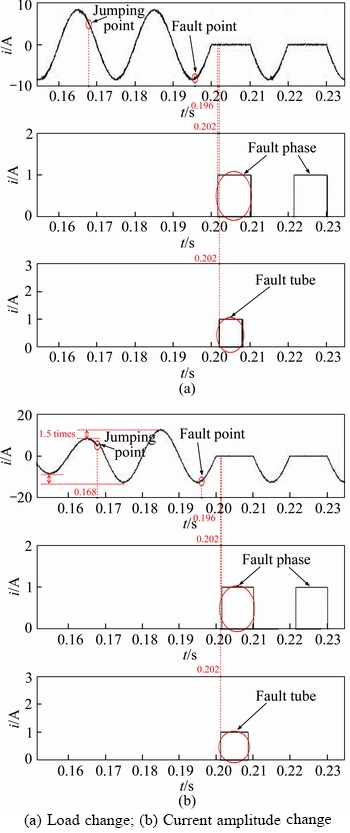
Figure 18 Experimental current waveform and fault diagnosis diagram of open circuit fault under condition of loads change:
Figure 19 shows two examples of SPWM- and SVPWM-based inverter. It can be seen that the method is well applicable to SPWM and SVPWM control strategies, and there is neither misjudgment nor false alarm in fault diagnosis process. Finally, V1 can be accurately located in half cycle.
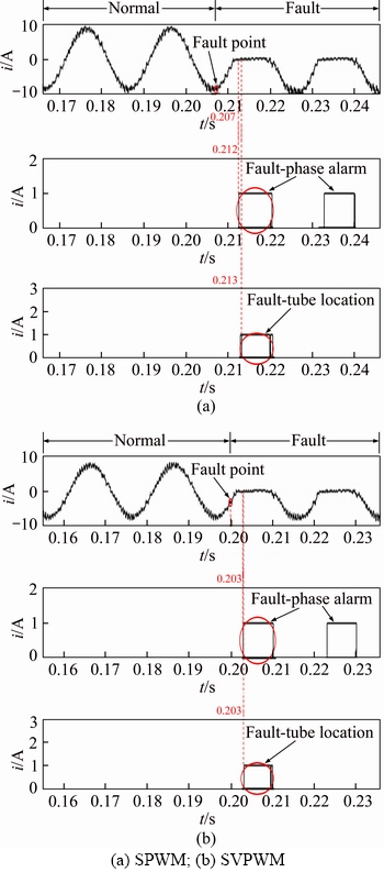
Figure 19 Experimental current waveform and fault diagnosis diagram of open circuit fault under different control strategies:
Moreover, when the phase current frequency or the carrier frequency increases, the diagnosis speed will also increase. The accuracy of the results will not be affected by frequency.
4.5 Limitation analysis
The proposed fault diagnosis method is based on the detection of the phase current. The foregoing specifies the principles and procedures of the specific implementation of the proposed method. In the experiment, considering the actual situation of the current fluctuations and interference, the detection of io(t)=0 is set with a threshold of 5% amplitude. Therefore, the actual setting is |io(t)|��0.4, and the detection of |io(t)|��0.4 installed 9 detection points, the time interval between each detection point is 0.0002 s (1% of the length of a cycle). In theory, 0.0016 s (2/25 of the length of a cycle) decision time is required from finding faults to identifying faults. Because there are settings to prevent false alarm, if the fault occurs within 0.0016 s before the critical point of the current direction change (hereinafter referred to as the changing point), and the direction of the transformation is exactly non-fault direction, then the fault cannot be warned in time in this situation. Take V1 and V2 fault analysis as examples, the specific waveform is shown in the following figure.
The V1 fault limitation analysis diagram is shown in Figure 20(a). It can be seen that there is a changing point of the instruction current at 0.19 s, and the change direction is the non-fault direction. The analysis of the V2 fault is consistent with the V1 process, and the conclusion is the same. The output current waveform and the fault detection diagram are shown in Figure 20(b). The fault setting time is 0.189 s, and it can be seen that the direction of expected current changes just 0.001 s after the fault occurs. As a result, the actual output current which tracks the instruction current remains very short time in interval (it is far below the 0.0016 s which is needed to ensure a failure occurs). After that, the output current enters the normal tracking interval, and a complete fault characteristic interval can be found in the next fault cycle. Therefore, the time of alarm and the location of the fault tube are respectively in 0.202 s and 0.203 s, and the time after the fault has passed is 0.013 s and 0.014 s (close to 3/4 cycle). This situation can cause a delay in diagnosis.
5 Conclusions
1) This paper proposes an on-line diagnosis method for open circuit fault of inverters. The accurate analytical model of power tube under open circuit fault condition is established. The three-phase bridge inverter circuit model with current hysteresis control is established on the basis of Matlab/simulink simulation platform.
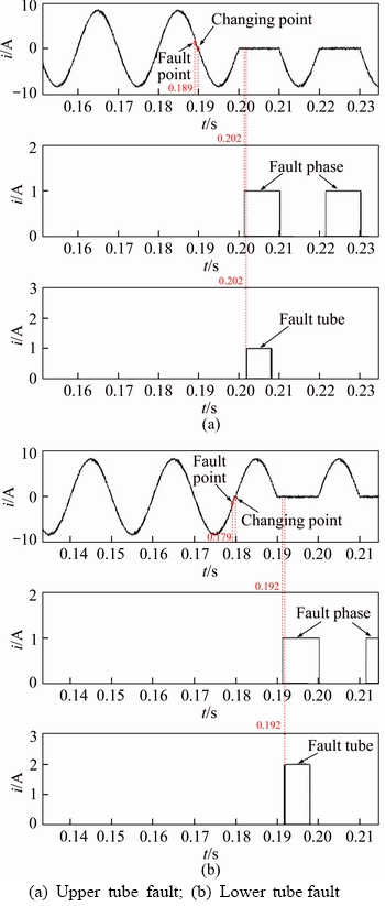
Figure 20 Experimental current waveform and fault diagnosis diagram of open circuit fault under condition of limitation analysis:
2) According to the output current io(t)=0 and the direction of output current tracking instruction current, two fault characteristics are jointly applied to diagnose and locate the fault. The proposed method is simple and easy to apply, and it is independent of system control signals or extra sensors, and has a short diagnosis time. Moreover, the proposed method can also be applied a variety of control strategies.
3) Finally, the validity, reliability and limitations of the diagnostic method are verified and analyzed on the dSPACE experiment platform.
References
[1] FRIEDRICH W F. Some diagnosis methods for voltage source inverters in variable speed drives with induction machines-A survey [C]// The 29th IECON. 2003: 1378�C1385. DOI: 10.1109/IECON.2003.1280259.
[2] YANG Shao-yong, BRYANT A, MAWBY P, XIANG Da-wei, RAN Li, TAVNER P. An industry-based survey of reliability in power electronic converters [J]. Industry Applications, 2011, 47(3): 1441�C1451. DOI: 10.1109/TIA. 2011.2124436.
[3] CHOI U M, BLAABJERG F, LEE K B. Study and handling methods of power IGBT module failures in power electronic converter systems [J]. Power Electronics, 2015, 30(5): 2517�C2533. DOI: 10.1109/TPEL.2014.2373390.
[4] YANG Shao-yong, XIANG Da-wei, BRYANT A, MAWBY P, RAN Li, TAVNER P. Condition monitoring for device reliability in power electronic converters: A review [J]. Power Electronics, 2010, 25(11): 2734�C2752. DOI: 10.1109/TPEL.2010.2049377.
[5] MA Hao, WANG Lin-guo. Fault diagnosis and failure prediction of aluminum electrolytic capacitors in power electronic converters [C]// The 31st IECON. 2005: 842�C847. DOI: 10.1109/IECON. 2005. 1569014.
[6] MASRUR M A, CHEN Z, MURPHEY Y. Intelligent diagnosis of open and short circuit faults in electric drive inverters for real-time applications [J]. Power Electronics, 2010, 3(2): 279�C291. DOI: 10.1049/iet-pel.2008.0362.
[7] QIANG Sheng, LI Ying-ying. Motor inverter fault diagnosis using wavelets neural networks [C]// IEEE International Conference on Systems. 2013: 3168�C3173. DOI: 10.1109/SMC.2013.540.
[8] HUANG Zhan-jun, WANG Zhan-shan, ZHANG Hua-guang. Multiple open-circuit fault diagnosis based on multistate data processing and subsection fluctuation analysis for photovoltaic inverter [J]. Instrumentation and Measurement, 2018, 67(3): 516�C526. DOI: 10.1109/TIM.2017.2785078.
[9] OMID N S, HUANG Biao. Bayesian control loop diagnosis by combining historical data and process knowledge of fault signatures [J]. Industrial Electronics, 2015, 62(6): 3696�C3704. DOI: 10.1109/TIE.2014.2375253.
[10] CAI Bao-ping, ZHAO Yu-bin, LIU Han-lin, XIE Min. A data-driven fault diagnosis methodology in three-phase inverter for PMSM drive systems [J]. Power Electronics, 2017, 32(7): 5590�C5600. DOI: 10.1109/TPEL.2016. 2608842.
[11] AN Qun-tao, SUN Li-zhi, ZHAO Ke, SUN Li. Switching function model-based fast-diagnostic method of open-switch faults in inverters without sensors [J]. Power Electronics, 2011, 26(1): 119�C126. DOI: 10.1109/TPEL.2010.2052472.
[12] ALAVI M, WANG Dan-wei, LUO Ming. Model-based diagnosis and fault tolerant control for multi-level inverters [C]// The 41st IECON. 2015: 1548�C1553. DOI: 10.1109/IECON.2015.7392321.
[13] ALAVI M, LUO Ming, WANG Dan-wei, ZHANG Dan-hong. Fault diagnosis for power electronic inverters: A model-based approach [C]// The 8th IEEE Symposium on Diagnostics for Electrical Machines, Power Electronics & Drives. Piscataway, NJ, USA: IEEE. 2011: 221�C228. DOI: 10.1109/DEMPED.2011. 6063627.
[14] ZHENG Hong, WANG Ruo-yin, WANG Yi-fan, ZHU Wen. Fault diagnosis of photovoltaic inverters using hidden Markov model [C]// The 36th Chinese Control Conference. 2017: 7290�C7295. DOI: 10.23919/ChiCC.2017.8028508.
[15] CHENG Shu, CHEN Ya-ting, YU Tian-jian, WU Xun. A novel diagnostic technique for open-circuited faults of inverters based on output line-to-line voltage model [J]. Industrial Electronics, 2016, 63(7): 4412�C4421. DOI: 10.1109/TIE.2016.2535960.
[16] ABADI M B, MENDES A M S, CRUZ S M  . Method to diagnose open-circuit faults in active power switches and clamp-diodes of three-level neutral-point clamped inverters [J]. Electric Power Applications, 2016 10(7): 623�C632. DOI: 10.1049/iet-epa.2015.0644.
[17] FREIRE N M A, ESTIMA J O, CARDOSO A J M. A voltage-based approach without extra hardware for open-circuit fault diagnosis in closed-loop PWM AC regenerative drives [J]. Industrial Electronics, 2014, 61(9): 4960�C4970. DOI: 10.1109/TIE. 2013.2279383.
[18] WU Xun, TIAN Rui, CHENG Shu, CHEN Te-fang, TONG Li. A nonintrusive diagnostic method for open-circuit faults of locomotive inverters based on output current trajectory [J]. Power Electronics, 2018, 33(5): 4328�C4341. DOI: 10.1109/TPEL. 2017.2711598.
[19] HE Jiang-biao, DEMERDASH N A O, WEISE N, KATEBI R. A fast on-line diagnostic method for open-circuit switch faults in SiC-MOSFET-Based T-type multilevel inverters [J]. Industry Applications, 2017, 53(3): 2948�C2958. DOI: 10.1109/TIA. 2016.2647720.
[20] YAN Hao, XU Yong-xiang, ZOU Ji-bin, FANG Yuan, CAI Fei-yang. A novel open-circuit fault diagnosis method for voltage source inverters with single current sensor [J]. Power Electronics, 2018, 33(10): 8775�C8786. DOI: 10.1109/TPEL. 2017.2776939.
[21] JLASSI I, ESTIMJ O A, KHIL E, KHOJET S, BELLAAJ N M, CARDOSO A J M. Multiple open-circuit faults diagnosis in back-to-back converters of PMSG drives for wind turbine systems [J]. Power Electronics, 2015, 30(5): 2689�C2703. DOI: 10.1109/TPEL. 2014.2342506.
[22] LU Bin, SHARMS K A. A literature review of IGBT fault diagnostic and protection methods for power inverters [J]. Industry Applications, 2009, 45(5): 1770�C1777. DOI: 10.1109/TIA. 2009. 2027535.
[23] LI Wei, LIU You-mei, CHEN Te-fang, DENG Jiang-ming. An adaptive stable observer for on board auxiliary inverters with online current identification strategy [J]. Journal of Central South University, 2017, 24: 819�C828. DOI: 10.1007/s11771-017-3484-y.
[24] WU Xun, CHEN Te-fang, CHENG Sshu, YU Tian-jian, XIANG Chao-qun, LI Kai-di. A noninvasive and robust diagnostic method for open-circuit faults of three-level inverters [J]. IEEE Access, 7: 2006�C2016. DOI: 10.1109/ ACCESS.2018.2886706.
[25] ESTIMJ O A, CARDOSO A J M. A new algorithm for real-time multiple open-circuit fault diagnosis in voltage-fed PWM motor drives by the reference current errors [J]. Industrial Electronics, 2013, 60(8): 3496�C3506. DOI: 10.1109/TIE.2012.2188877.
[26] ABRAHAMSEN F, BLAABJRG F, RIES K, RASMUSSEN H. Fuse protection of IGBTs against rupture [C]// Nordic Workshop Power Industrial Electronics. 2004: 611�C615.
(Edited by FANG Jing-hua)
���ĵ���
���ڵ����켣���������·�������߹�����ϵ�һ���·���
ժҪ��������İ�ȫ����ɿ����ǵ�������ϵͳ�ȶ����еIJ��ɻ�ȱ����������������Ĺ��ϴ��������еĿ���Ԫ�������й���������ġ��������ͻ��������Ƶ��������Ϊ�о����������һ�ֿ������ڸ��ֿ��Ʋ����µĿ�·������Ϸ�����������Ŀ�·���ϻᵼ�������������䣬�ɽ���������Ϊһ����������������ϱȽϹ��Ϸ���ǰ�������������ʵ���ڰ�������ڶԿ�·���ϵ���ϼ���λ�����⣬����Ϸ����Ȳ���Ҫ��ȡϵͳ�����źţ�Ҳ����Ҫ���Ӷ�����������ͨ��dSPACE��ʵ��ʵ��ƽ̨�����������������Ч�ԡ��ɿ��Լ������Խ�������֤�ͷ�����
�ؼ��ʣ�������ϣ��ͻ�������������϶�λ
Foundation item: Projects(2016YFB1200401, 2017YFB1200801) supported by the National Key R & D Program of China
Received date: 2018-07-16; Accepted date: 2019-01-17
Corresponding author: CHENG Shu, PhD, Professor; Tel/Fax: +86-10-82656800; E-mail: 6409020@qq.com; ORCID: 0000-0002-0709- 6960
Abstract: Security and reliability of inverter are an indispensable part in power electronic system. Faults of inverter are usually caused by switch elements�� operating fault. Taking the inverter with hysteresis current control as the research object, a universal open-circuit fault location method which can be applied to multiple control strategies is proposed in the paper. If the switch open-circuit fault happens in inverter, the output phase current will inevitably change, which can be used as a characteristic for diagnosis, combined with the comparison of phase-current direction before and after the fault occurrence, to diagnose and locate the open-circuit fault in a half cycle. Moreover, this method requires neither system control signals nor sensor. The validity, reliability and limitation of the fault location method in the paper are verified and analyzed through dSPACE-based experiment platform.
