

J. Cent. South Univ. (2020) 27: 2643-2661
DOI: https://doi.org/10.1007/s11771-020-4488-6

A unified approach of PID controller design for unstable processes with time delay
Ashraf RAZA, Md Nishat ANWAR
Electrical Engineering Department, National Institute of Technology, Patna-800005, India
 Central South University Press and Springer-Verlag GmbH Germany, part of Springer Nature 2020
Abstract:
This paper addresses a unified approach of the PID controller design for low as well as high order unstable processes with time delay. The design method is based on the direct synthesis (DS) approach to achieve the enhanced load disturbance rejection. To improve the servo response, a two-degree of freedom control scheme has been considered. A suitable guideline has been provided to select the desired reference model in the DS scheme. The direct synthesis controller has been approximated to the PID controller using the frequency response matching method. A consistently better performance has been obtained in comparison with the recently reported methods.
Key words:
Cite this article as:
Ashraf RAZA, Md Nishat ANWAR. A unified approach of PID controller design for unstable processes with time delay [J]. Journal of Central South University, 2020, 27(9): 2643-2661.
DOI:https://dx.doi.org/https://doi.org/10.1007/s11771-020-4488-61 Introduction
Unstable system contains at least one pole in the right half of s-plane and is found in different chemical processes such as polymerization reactors, heat exchangers. These processes are difficult to control as compared to the stable processes. In the last decade, researchers have given more attention towards the PID controller design for unstability with time delay system. PID controller is most widely used in process industries due to its simplicity, low cost and satisfactory performance for a variety of processes and more than 90% process industries use PI/PID controllers. But tuning of PI/PID controllers for unstable processes with process uncertainties is a difficult task due to the presence of the time delay term and the improper tuning may lead to poor robustness and large oscillatory responses [1]. Therefore, these problems should be rectified to get enhanced performance. Many tuning rules have been proposed for the time delayed unstable process based on the internal model control (IMC) [2-10] or the direct synthesis (DS) [11-15] methods.
VANAVIL et al [2] designed IMC based PID controller with lead-lag filter for first order unstable and integrating processes. SHAMSUZZOHA et al have designed IMC based PID controller with lead/lag filter for unstable first order plus dead time (UFOPDT) [3] and unstable second order plus dead time (USOPDT) [4] processes. YANG et al [5] designed IMC based controller either in PID or in higher order form for the unstable processes with one RHP pole only. An IMC-PID controller for integrating and unstable with time delay system is proposed by KUMAR et al [6] using the Pade��s approximation of the time delay term whereas SHAMSUZZOHA [7] proposed a unified PID controller design for both the stable and unstable (with one unstable pole) processes based on the disturbance rejection in the IMC control scheme. PANDA [8] proposed a PID controller design for low order unstable processes using the Laurent series expansion of the controller function in the IMC scheme. WANG et al [9] proposed an IMC PID tuning rule for integrating and unstable processes (one RHP pole) with time delay by introducing an imaginary first order filter based on pole zero conversion whereas BEGUM et al [10] designed an IMC-based analytical PID tuning rule for UFOPDT process with the desired robustness level (the maximum sensitivity, Ms) for different time delay to time constant ratios in which the tuning parameter is also based on the maximum sensitivity function. Similarly, SHAMSUZZOHA [16] designed IMC based PID controller for time delay stable and unstable (with one unstable pole) processes with the criterion of the maximum sensitivity.
RAO et al [11] designed DS-based PID controller in series with a lead-lag filter for unstable second order process with time delay by considering the two tuning parameters in two degrees of freedom (DoF) control scheme whereas VANAVIL et al [12] designed DS based PID controller with a lead-lag filter for first order and second order unstable process with dead time by the second order Pade��s approximation of the dead time term. BABU et al [13] used DS method to design PID controller for UFOPDT and USOPDT process by comparing the closed loop characteristic equation with the desired characteristic equation. CHO et al [14] designed PID controller for the basic control structure with the set point filter to have two degrees of freedom control scheme for different types of unstable processes by approximating the time delay term and the model reduction of the higher order processes. The performance of the set-point and the load disturbance changes of PID controller developed by CHO et al [14] for unstable systems is analyzed by BEGUM et al [15] through DS-IAE based index for the step and the ramp input.
To improve the performance in the set-point tracking and the load disturbance rejection of the unstable process, a complex two-degree of freedom control structure with more number of controllers was used in Refs. [17-19]. LIU et al [17] proposed a two-degree of control structure which decouples the set-point and the load disturbance response performance by the set-point tracking controller and the disturbance estimator. In addition to the set-point tracking controller, an auxiliary controller (proportional or proportional-derivative controller) is also used for stabilizing the set-point response. Both the controllers are designed by minimizing the ISE (integral square error) performance specification and the resulting controllers are either PID or the higher order controller. To enhance the performance of the unstable process without the higher order controller, SHAMSUZZOHA et al [18] designed an IMC based PID controller with a lead-lag filter for the disturbance estimator in the same control structure as proposed by LIU et al [17]. Recently AJMERI et al [19] proposed a modified two-degree of freedom parallel control structure (PCS) for the improved performance of the unstable processes with small time delay and the PI/PID controller is designed using the direct synthesis method. But for the unstable process with normalized time delay greater than one, this PI/PID controller fails to give the satisfactory performance in spite of complex structure and more number of controllers.
In addition to the above design methods, some authors designed the controller for unstable processes which are different from the DS and IMC based methods. Based on the Smith predictor control scheme, CONG et al [20] used the double loop control model for the control of unstable processes (one RHP pole) in which the inner loop is used to stabilize the process and the outer loop is used to enhance the set-point performance and for the load-disturbance performance, a disturbance controller is used. NIKITA et al [21] designed PID controllers for USOPDT system using the relay auto-tuning method by calculating the ultimate gain of the controller. CHEN et al [22] proposed a set-point weighted PID controller for unstable processes with time delay, showing that set-point weighted PID controller is equivalent with a PD controller in the inner loop in addition to PID controller.
The present work of the controller design is based on the direct synthesis method and the selection of the reference model (desired closed loop transfer function). The following points are considered in designing the controller for the unstable processes.
1) The control structure should be simple such as the classical unity negative feedback configuration.
2) The design of the controller is such that it can be uniformly applied to the low order as well as high order processes with any number of unstable and/or stable poles.
3) The designed controller can be applied both for the small and large time delay systems without approximation of the time delay term.
4) There is a generalized reference model for all types of unstable processes depending upon the number of pole-zero cancellations.
The controller design through DS method may be a higher order controller and sometimes may not be physically realizable. Therefore, the DS controller is approximated into a PID controller using the two low frequency points in the frequency response matching. To reduce the overshoot in the set-point response, a set-point filter is designed according to the selected reference model transfer function leading to two-degree of freedom (2DoF) control.
For clear interpretation, the proposed work is organized as follows. The design method is discussed in Section 2 whereas in Section 3 the simulation of the proposed method and the comparison with the recently reported method for different types of unstable process are carried out. The robustness analysis and the conclusion of the work are addressed in Sections 4 and 5 respectively.
2 Design method
Consider an unstable process which is described by the transfer function,
 (1)
(1)
where N(s)/D(s) is the rational part of the transfer function and L is the time delay of the process. The simple control structure in unity negative feedback configuration is considered, as shown in Figure 1.
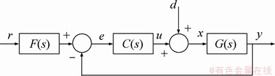
Figure 1 Classical unity negative feedback closed loop configuration
where C(s) is the controller and F(s) is a set-point filter; r is the reference input; e is the error; u is the manipulated variable; d is the disturbance; y is the controlled variable of the process.
The controller design is described below without the set-point filter F(s). The closed-loop transfer function from the input r to the output y is given as
 (2)
(2)
In the direct synthesis (DS) method, the controller design is based on the process model and a desired closed-loop transfer function. The closed-loop transfer function for the desired set-point response is selected as Gr,y(s). The controller C(s), which will yield the desired response, may be obtained as
 (3)
(3)
In the case of unstable processes, the controller C(s) must not have zero to cancel the unstable pole/s of the process G(s) or in other words, the controller must have pole zero cancellation at least at the unstable poles of the process. This can be achieved by the proper selection of the desired reference model Gr,y(s) for a particular process. The selection of the reference model for the unstable processes with dead time is generalized as follows:
 (4)
(4)
where p is the number of poles of the process for the pole zero cancellation in the controller C(s); �� is the only tuning parameter which is the time constant or the response speed of the reference model. The detail discussion of the selection of the reference model and the value of �� for particular type of the unstable process is as follows.
Case 1: UFOPDT process. Consider an unstable first order plus dead time (UFOPDT) process with transfer function given by
 (5)
(5)
where T is the time constant; K is the gain; L is the time delay of the process. Here the value of p is equal to 1. So, the reference model is selected as
 (6)
(6)
where �� is the tuning parameter which is the desired closed-loop time constant and �� is selected in such a way to avoid the unstable pole zero cancellation. Now from Eq. (3), the controller C(s) may be written as
 (7)
(7)
where �� and �� are selected such that
 (8)
(8)
which gives the �� as
 (9)
(9)
Case 2: USOPDT process with one unstable pole. Consider an unstable second order plus dead time (USOPDT) process with transfer function given by
 (10)
(10)
The reference model may be selected as below if only unstable pole is considered for pole-zero cancellation in C(s).
(11)
where �� and �� are selected in the same manner as those in the UFOPDT process such that
 (12)
(12)
which gives the �� as
 (13)
(13)
But sometimes the time constant T2 is so large that it causes sluggish response. So, it is recommended to have pole-zero cancellation of the controller at unstable as well as stable poles. So, here the value of p is equal to 2 and the reference model may be selected as
 (14)
(14)
From Eq. (3), C(s) may be written as
 (15)
(15)
where �� and �� are selected in such a way that
 (16)
(16)
The values of ��1 and ��2 may be obtained from Eq. (16) as below,
 (17)
(17)
Case 3: USOPDT process with two unstable poles. Consider an unstable second order process with two unstable poles as given by
 (18)
(18)
where the value of p is equal to 2. So, the reference model is selected as
 (19)
(19)
Now from Eq. (3), C(s) may be written as
 (20)
(20)
where �� and �� are selected in such a way that
 (21)
(21)
The values of ��1 and ��2 may be obtained from Eq. (21) as below.
 (22)
(22)
Case 4: Higher order process with time delay. For the higher order process, the same procedure is applied as above. The reference model for the process with poles at q1, q2, ��, qp (stable or unstable) may be taken as (when all the poles of the process have pole-zero cancellation in the controller C(s)):
(23)
The controller C(s) may be written as
 (24)
(24)
The values of �� and �� are selected in such a way that the closed loop expression will avoid the pole-zero cancellation between the process model and the controller especially on the unstable pole. This can be achieved by cancelling the zeros at the poles of the process in the controller expression of Eq. (24). Thus the following expression is obtained so that the denominator of the controller expression also has poles at the same location as the poles of the process.
 (25)
(25)
The different �� may be obtained from Eq. (25) and written in the matrix form as below:
 (26)
(26)
The DS controller C(s), obtained from Eq. (3), may be a higher-order controller and may not be practically realizable. Therefore, the PID controller CPID(s) is considered in the parallel form which is the most commonly used controller in the process industries and is given by
 (27)
(27)
where KP, KI and KD are the proportional, the integral and the derivative gains, respectively. To match the direct synthesis controller C(s) by the PID controller CPID(s), the frequency response matching of the two controllers is considered [23, 24] as given below,
 (28)
(28)
 (29)
(29)
where and
and
 .
.
Separating the real and imaginary parts from Eq. (29), the following expression may be obtained.
 and
and  (30)
(30)
Expanding the expressions of Eq. (30) by Taylor series expansion about ��=0 and equating the initial R derivatives of the corresponding functions, the following equations may be obtained.
 (31)
(31)
 (32)
(32)
where
Using the divided difference calculus [25], the above relations can be simplified to the following algebraic equation:
 (33)
(33)
and
 (34)
(34)
where ��m are very small positive values near zero.
From Eqs. (33) and (34) at least two frequency points (��0 and ��1 around ��=0) are needed for evaluating the 3 unknown parameters of the PID controller. The real part of left hand side expression of Eq. (33) has only one parameter KP, hence two values of KP are obtained for the two low frequency points as given by KP1=CR(��0); KP2=CR(��1).
It is observed from various examples that KP1��KP2 and we may take an average of these as
 (35)
(35)
Hence, to evaluate KI and KD, Eq. (34) may be simplified for the two low frequency points as
 (36)
(36)
where,

 and
and 
Then, solution of Eq. (36) determines KI and KD as
 (37)
(37)
 (38)
(38)
Thus, the parameters of the PID controller are evaluated from Eqs. (35), (37) and (38).
The tuning rule is summarized in Tables 1 and 2.
Table 1 Summary of selection of reference model, �� terms and set-point filter
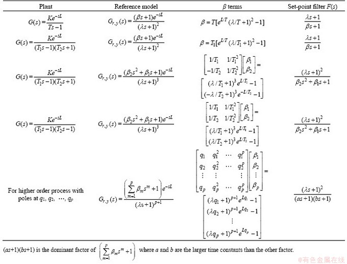
Table 2 Parameters of PID controller
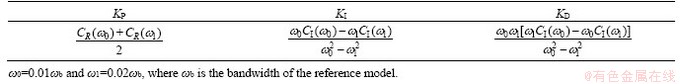
Selection of low frequency points: The close matching of the designed system with the desired closed-loop system is obtained by good approximation of C(s) by the CPID(s). Thus the small values of frequency points are chosen at around 1% of the bandwidth frequency (��b) of the desired reference model. The closer matching in the low frequency region is more important since most industrial processes show low-pass dynamics in the frequency response. These are observed through simulation which gives good result for most of the processes. Here, the frequency value has been chosen as ��0=0.01��b and ��1= 0.02��b.
3 Simulation results
To show the performance of the proposed method, simulation has been carried out on different unstable processes with time delay. It is also compared with some of the well-known methods recently reported in the literature by considering the robustness level measured by the maximum sensitivity (Ms). The set-point filter is used to reduce the overshoot in the set-point response. Different performance parameters such as IAE (integral absolute error) for the output performance and TV (total variation) value for the smoothness of the controller output or the manipulated variable are calculated to evaluate the proposed PID controller. To avoid the derivative kick in the derivative term of the PID controller, a derivative filter (DF) of first order lag is used in all the simulation. The time constant (Tf) of the DF is taken as Tf=��Td, where Td=KD/KP and Td is the derivative time constant. The value of ��=0.01 is chosen not for bias of the results, but for high noisy processes, so a large value of �� in the range of 0.1-0.2 may be used [26].
Selection of the tuning parameter ��: The tuning parameter is selected such that it gives good disturbance rejection and good robustness but these two conditions are contradictory to each other since for good disturbance rejection the tuning parameter should be small but at small value of �� the robustness will be poor and vice-versa. The robustness is measured by the maximum sensitivity (Ms) which is the inverse of the shortest distance from the point (-1, 0) to the Nyquist plot of the loop transfer function. For robust stable system the value of Ms may vary in the range of 1.2-2.0 but for unstable systems this value may be larger than 2. For the selection of the tuning parameter �� for the unstable process, a curve is plotted between �� and Ms for all the examples. The value of �� is selected in the negative slope region after the peak value of Ms since the selection of the tuning parameter before the peak value (or in the positive slope region) may cause the system to be unstable. To have a good tradeoff between the disturbance rejection and the robustness, a suitable value in the range of negative slope region (typically between the two extreme values of �� in the negative slope region) is selected. The value of Ms can also be related to the gain margin (GM) and phase margin (PM) as GM��Ms/(Ms-1), PM��2sin-1(1/2Ms) [27].
Example 1: Consider an unstable first order plus dead time (UFOPDT) process taken from CHO et al [14] as given by  .
.
For proper selection of ��, the graph is plotted for Ms against �� as shown in Figure 2. From Figure 2, the value of �� is selected after the peak since before the peak value of Ms the closed loop system may become unstable for even a small disturbance. Therefore, �� should be taken greater than 0.1 for stable responses (as the peak value occurs at ��=0.1) preferably in the negative slope region of the plot (0.1<��<1.5). The selection of �� is very important and there is always a tradeoff in robustness and performance of the closed-loop system.
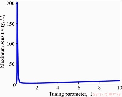
Figure 2 Plot of maximum sensitivity Ms with tuning parameter �� for Example 1
For better performance and robustness trade-off, the tuning parameter �� is selected as 0.85 (in between 0.1 and 1.5) in the proposed method which gives Ms=2.36 and the simulation results are compared with that of CHO et al [14] and SHAMSUZZOHA [7]. The controller parameters, the robustness parameter Ms and the performance indices of all the methods are tabulated in Table 3. The set-point as well as the load disturbance responses of the proposed method compared with CHO et al [14] and SHAMSUZZOHA [7] is shown in Figures 3-6. The proposed method gives significant improvement over both the methods even for the low value of Ms. SHAMSUZZOHA [7] and CHO et al [14] have already shown its superior performance to many other methods in the literature.
Table 3 Controller parameters and performance indices of nominal and perturbed system for Example 1
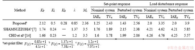
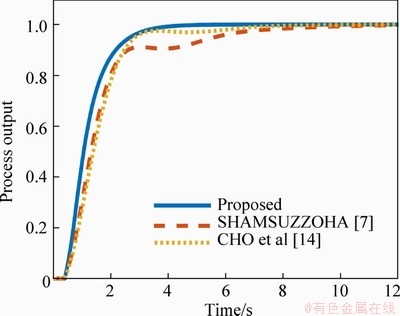
Figure 3 Process output of set-point response for Example 1
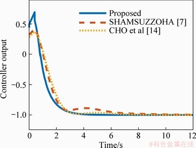
Figure 4 Controller output of set-point response for Example 1
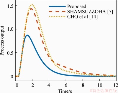
Figure 5 Process output of load disturbance response for Example 1
To show the robust performance of the controller, a 10% change in both the gain and the time-delay is considered simultaneously and the step response and the controller output are shown in Figures 7 and 8 respectively. It can be observed that the proposed method gives significant improvement in the response over the other methods and the performance indices for the perturbed system tabulated in Table 3 show less IAE and TV values than the other two methods. The TV value of the proposed method is slightly higher for the set-point response.
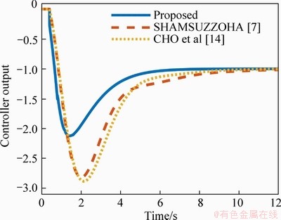
Figure 6 Controller output of load disturbance response for Example 1
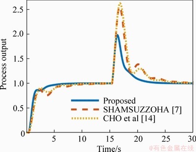
Figure 7 Process output of perturbed system for Example 1
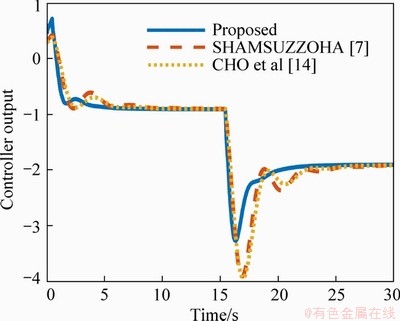
Figure 8 Controller output of perturbed system for Example 1
Example 2: Consider an unstable first order plus dead time (UFOPDT) delay dominant process taken from CHO et al [14] as given by

For stable system, the process is delay dominant if (��/��)>5; but for unstable system, the process is delay dominant if (��/��)>1 due to sensitivity to the change even for small value of time delay [2].
The plot of the maximum sensitivity Ms with �� is shown in Figure 9. The tuning parameter �� is selected after both the peaks of Ms and preferably in the negative slope region (1.6<��<4) of the plot.
The parameters of the controller and the different performance indices are tabulated in Table 4 and the simulation results are shown in Figures 10-13 for both the servo and the regulatory response. For the set-point tracking, AJMERI et al [19] gave the best response but at the cost of complex control structure with more number of controllers. In the load-disturbance rejection, the proposed method gives better response than the other methods, which shows superiority of the proposed method.
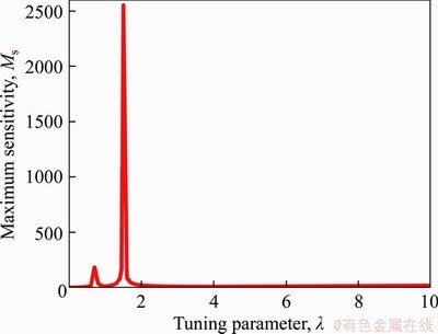
Figure 9 Plot of maximum sensitivity Ms with tuning parameter �� for Example 2
To show the robustness of the controller design, a 5% change in the dead time of the process is considered as it is very sensitive to change in the time delay for delay dominant unstable system. The simulation results for the perturbed system are shown in Figures 14 and 15, which shows satisfactory performance of the proposed controller design.
Example 3: Consider a third-order delayed unstable process with one unstable pole taken from SHAMSUZZOHA [7] as given by G3(s)= SHAMSUZZOHA [7] and other authors applied the tuning rule by reducing the above process into second order delayed unstable process using SKOGESTAD [26] method which is given by
But the proposed tuning rule can be applied both for the second and the higher order (in this case third order) process models and the proposed controller designs for both the models are compared with the other methods. In the proposed method, the pole-zero cancellation of the controller C(s) is carried out both for stable and unstable poles of the process. If the pole-zero cancellation is carried out only for the unstable pole it causes sluggish response in the load disturbance rejection if the stable pole has dominant time constant. The plot of the maximum sensitivity Ms with �� for the proposed method is shown in Figure 16 for both the third-and second-order model.
The tuning parameter �� is chosen after the peak value of Ms in the negative slope region (1.1<��<2.5) for the third-order model and at ��=1.89, Ms is equal to 2.2 which is the same robustness level as that in Ref. [7]. For the second-order model, the tuning parameter is selected in the negative slope region (1.2<��<5). For ��=2.67, Ms=2.2 is found for the proposed second-order model.
Table 4 Controller parameters and performance indices of nominal and perturbed system for Example 2
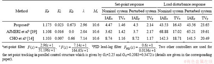
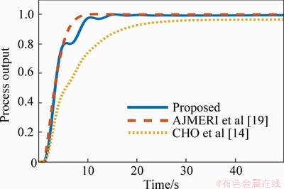
Figure 10 Process output of set-point response for Example 2
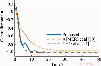
Figure 11 Controller output of set-point response for Example 2
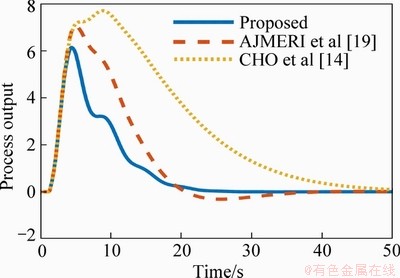
Figure 12 Process output of load disturbance response for Example 2
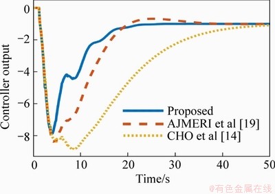
Figure 13 Controller output of load disturbance response for Example 2
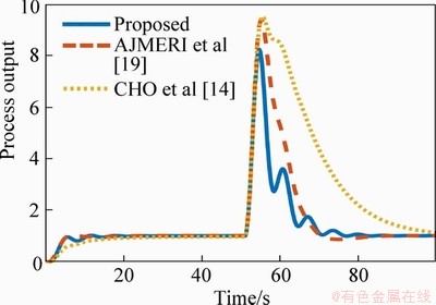
Figure 14 Process output of perturbed system for Example 2
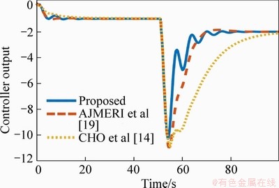
Figure 15 Controller output of perturbed system for Example 2
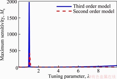
Figure 16 Plot of maximum sensitivity Ms with tuning parameter �� for Example 3
The controller parameters and different performance indices of different methods are tabulated in Table 5 for comparison. The simulation results are shown in Figures 17-20, which shows that the proposed method for both the second-and third-order models is comparable to the SHAMSUZZOHA [7] method and better than the YANG et al [5] method.
Table 5 Controller parameters and performance indices of nominal and perturbed systems for Example 3
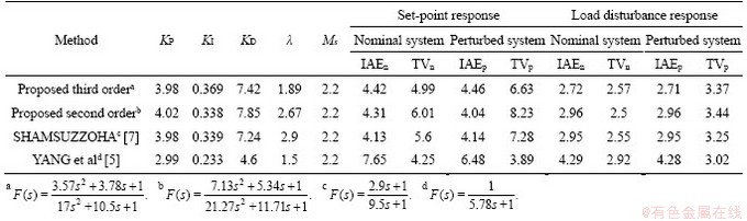

Figure 17 Process output of set-point response for Example 3

Figure 18 Controller output of set-point response for Example 3
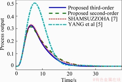
Figure 19 Process output of load disturbance response for Example 3
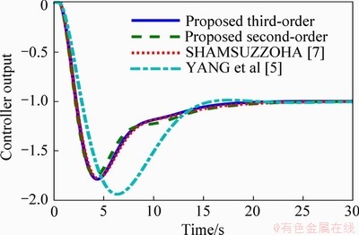
Figure 20 Controller output of load disturbance response for Example 3
To show the robustness of the proposed controller design a 20% change in both the gain and the dead time are considered. The simulation results of the perturbed process are shown in Figures 21 and 22 for the process and the controller output, which shows better performance than YANG et al [5] method and comparable to SHAMSUZZOHA [7] method.
Example 4: Consider a second-order delayed unstable process with two unstable poles taken from CHO et al [14] as given by:
 .
.
For choosing the tuning parameter ��, a plot of the maximum sensitivity Ms with respect to the tuning parameter is plotted as shown in Figure 23. The value of �� is chosen after the peak and the range of the �� for which the closed loop system will be stable from 0.5 to 2 (negative slope region). The proposed method is compared with the methods of CHO et al [14] and SHAMSUZZOHA et al [18] for the same robustness level of 2.33. The tuning parameter for the proposed method is selected as 1.22 to give Ms=2.33.
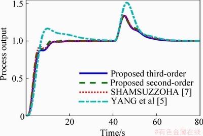
Figure 21 Process output of perturbed system for Example 3
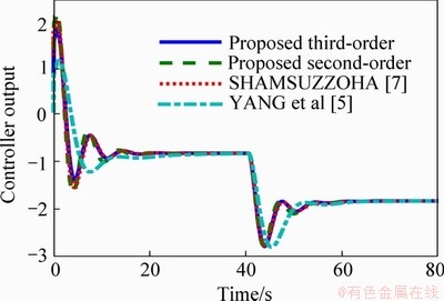
Figure 22 Controller output of perturbed system for Example 3
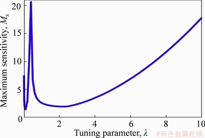
Figure 23 Plot of maximum sensitivity Ms with tuning parameter �� for Example 4
The controller parameters and the performance indices for Example 4 are tabulated in Table 6 and the simulation results are shown in Figures 24-29 for both the nominal and the perturbed systems. From Figures 24 and 25, it can be seen that SHAMSUZZOHA et al [18] method gives the best set-point response but with a very large TV value and the proposed method gives the comparable performance as compared to CHO et al [14] method. SHAMSUZZOHA et al used different controller for the set-point tracking and the load-disturbance rejection in a complex control structure. From Figures 26 and 27, the load disturbance response for the proposed method is better than the SHAMSUZZOHA et al [18] method and is comparable to the CHO et al [14] method.
For the perturbed system, a 20% change in both the gain and the dead time is considered simultaneously. The simulation results for the perturbed system are shown in Figures 28 and 29, which shows better performance for the proposed method as compared to the other two methods.
Example 5: Consider a pure integrating with time delay process as given by the following:
 .
.
The above process may be approximated by an unstable FOPDT as a worst case by considering the unstable pole very near to zero which is given below:
 .
.
The tuning parameter �� is chosen from the plot of Ms vs �� after the peak value of Ms (in the negative slope region) which is shown in Figure 30.
Table 6 Controller parameters and performance indices of nominal and perturbed system for Example 4
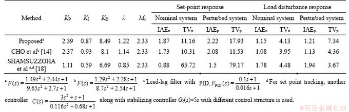
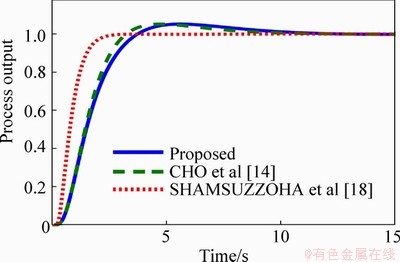
Figure 24 Process output of set-point response for Example 4
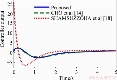
Figure 25 Controller output of set-point response for Example 4
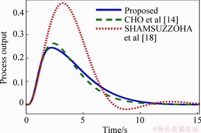
Figure 26 Process output of load-disturbance response for Example 4
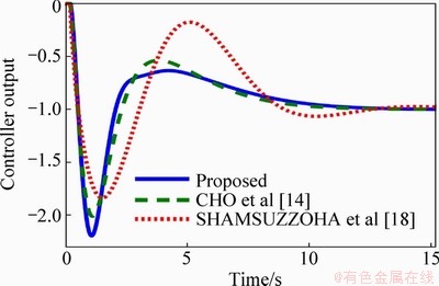
Figure 27 Controller output of load-disturbance response for Example 4
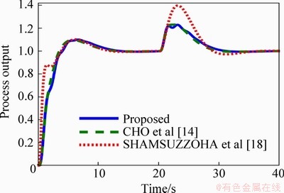
Figure 28 Process output of perturbed system for Example 4
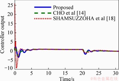
Figure 29 Controller output of perturbed system for Example 4
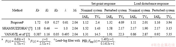
The proposed method is compared with the methods of SHAMSUZZOHA [7] and VANAVIL et al [2] for the same robustness level (Ms=2.04) and the simulation results for the nominal and the perturbed systems are shown in Figures 31-36. Also, the controller parameters and performance indices of the nominal and the perturbed systems for different methods are tabulated in Table 7 for comparison. The set-point performance for the proposed method is better than the other two methods as shown in Figure 31 and the controller output for the proposed method is slightly higher than the SHANSUZZOHA [7] method but is better than the VANAVIL et al [2] method as shown in Figure 32.
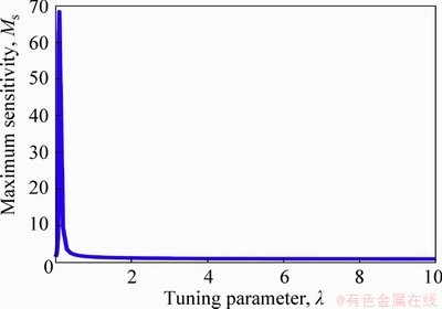
Figure 30 Plot of maximum sensitivity Ms with tuning parameter �� for Example 5
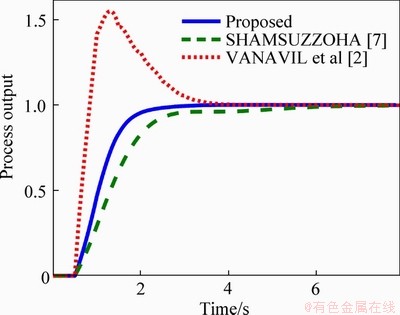
Figure 31 Process output of set-point response for Example 5
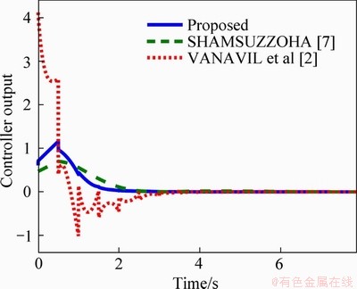
Figure 32 Controller output of set-point response for Example 5
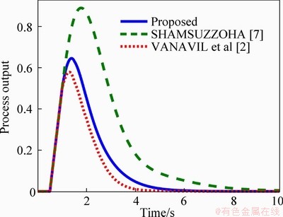
Figure 33 Process output of load-disturbance response for Example 5
The load-disturbance rejection of the proposed method is better than the SHAMSUZZOHA [7] method and comparable to VANAVIL et al [2] method but VANAVIL et al [2] method produces some spikes in the controller output and thus the TV value becomes large in the set-point response.
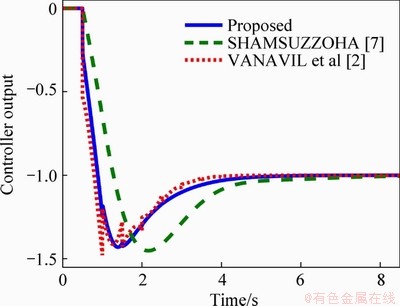
Figure 34 Controller output of load-disturbance response for Example 5
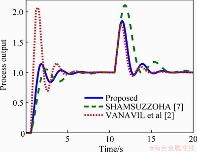
Figure 35 Process output of perturbed system for Example 5
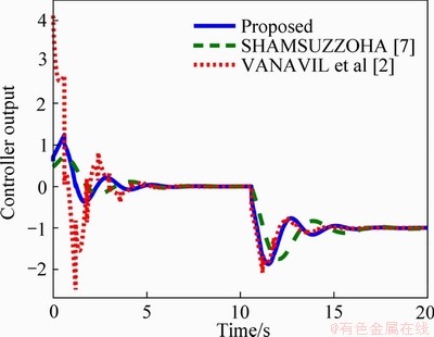
Figure 36 Controller output of perturbed system for Example 5
For analyzing the robustness of the controller, a 20% change in both the gain and the dead time is considered and the simulation results show that the proposed method gives better performance than the other two methods.
Example 6: Consider an unstable with integrating plus dead time process (UIPDT) taken from CHO et al [14] as given by the following:
 .
.
The integrating term of the above process may be approximated by an unstable first order term by considering the unstable pole very near to zero as given by the following expression:
 .
.
The tuning parameter �� is chosen from the plot of Ms vs �� shown in Figure 37 after the peak value of Ms and in the negative slope region (��=0.4 to 2.8).
Table 7 Controller parameters and performance indices of nominal and perturbed system for Example 5
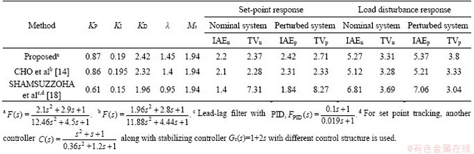
The proposed method is compared for the same robustness level (Ms=1.94) as that of CHO et al [14] and SHAMSUZZOHA et al [18] methods for fair comparison. The simulation results for the nominal and the perturbed systems are shown in Figures 38-43. The controller parameters and the performance indices for different methods are tabulated in Table 8 for comparison.
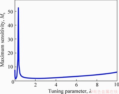
Figure 37 Plot of maximum sensitivity Ms with tuning parameter �� for Example 6
SHAMSUZZOHA et al [18] method gives slightly improved performance in the set-point response than the other two methods but at the cost of high TV value and the complex control structure which uses three different controllers. In the load-disturbance rejection of the nominal system, the performances of the proposed and the CHO et al [14] methods are comparable to each other and better than the SHAMSUZZOHA et al [18] method for both the process and the controller output.
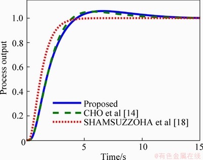
Figure 38 Process output of set-point response for Example 6
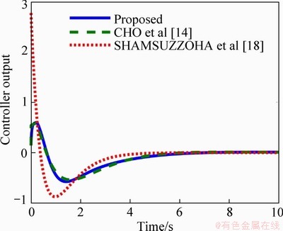
Figure 39 Controller output of set-point response for Example 6
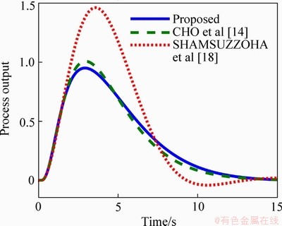
Figure 40 Process output of load disturbance response for Example 6
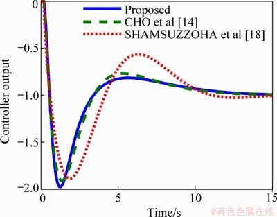
Figure 41 Controller output of load disturbance response for Example 6
For the perturbed system, a 20% change in both the gain and the dead time is considered and the simulation results for the process and the controller output are shown in Figures 42 and 43 respectively. This shows that the performance of the perturbed system of the proposed and the CHO et al [14] methods are comparable to each other and are better than the SHAMSUZZOHA et al [18] method.
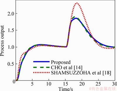
Figure 42 Process output of perturbed system for Example 6
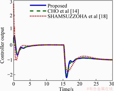
Figure 43 Controller output of perturbed system for Example 6
4 Robustness and stability analysis
The controller is designed using the nominal process model and the process model may be an approximation of the actual system dynamics. Therefore, it is necessary to check the robustness and stability of the control system in the presence of model uncertainties (here the parametric uncertainties such as gain uncertainty, uncertainties in time delay or in time constant are considered). Under these perturbed conditions, if the closed loop performance is good and stable, then the controller is said to be robust controller. The closed loop control system is said to be robustly stable system if and only if [28]
 (39)
(39)
where wm (s=j��) defines the bound on the process multiplicative uncertainty which is represented as
 .
.
And Tc(j��) is the closed loop complementary sensitivity function and from Figure 1 this may be written as
 .
.
where C(j��) is the controller and G(j��) is the nominal process model used to design the controller. Gp(j��) is the perturbed process.
Table 8 Controller parameters and performance indices of nominal and perturbed system for Example 6
For the unstable process if uncertainty exists in time delay (uncertainty of ��L), then to achieve robust stability condition as in Eq. (39), the tuning parameter for the controller design is selected such that
 (40)
(40)
If the uncertainty of ��K exists in the process gain, then multiplicative uncertainty bound may be written as, wm(s)=|��K/K| and the controller is tuned such that the robust stability constraint can be figured out as
 (41)
(41)
If the uncertainty exists in both the gain (��K) and the dead time (��L) which may be converted to the multiplicative uncertainty as wm(s)= and the controller is tuned to fulfil the robust stability constraint as
 (42)
(42)
The robust stability is checked for Example 1 for 20% uncertainty in both the gain and the dead time and is shown in Figure 44, which shows that the designed controller satisfies the robust stability constraint given by Eq. (42).
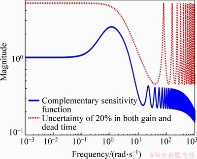
Figure 44 Plots of complementary sensitivity function and uncertainty of 20% in both gain and dead time for Example 1
Also to ensure the robust performance of the closed loop system for the disturbance rejection, the complementary sensitivity and sensitivity function must satisfy the following constraint [28]:

 (43)
(43)
where wp(j��) is the bound (or weight) on the sensitivity function Ts(s)=1-Tc(s). Therefore, the controller is tuned such that both the robust stability and the robust performance condition given by Eq. (39) and Eq. (43) should satisfy.
5 Conclusions
In this paper, a frequency domain PID controller design for the unstable system is proposed in the simple unity negative feedback configuration. The proposed method is based on the direct synthesis method and a unified approach is applied for all types of unstable processes. The proposed design method is free from the approximation of the time delay term and is applicable for the lower order as well as the higher order unstable system. A systematic way is followed for choosing the reference model and the set-point filter. The set-point filter is used to reduce the overshoot in the set-point response for a two- degree of freedom control scheme and is designed directly from the reference model transfer function. Simulation of different examples shows the effectiveness of the proposed method. Although the controller is designed for the unstable system, the procedure may be applied universally for stable and unstable systems.
References
[1] ASTROM K J, HAGGLUND T. Advanced PID control [M]. North Carolina: ISA Society, Research Triangle Park, 2006.
[2] VANAVIL B, ANUSHA A V N L, PERUMALSAMY M, RAO A S. Enhanced IMC-PID controller design with lead-lag filter for unstable and integrating processes with time delay [J]. Chem Eng Commun, 2014, 201: 1468-1496.
[3] SHAMSUZZOHA M, LEE M. Analytical design of enhanced PID filter controller for integrating and first order unstable processes with time delay [J]. Chem Eng Sci, 2008, 63: 2717-2731.
[4] SHAMSUZZOHA M, LEE M. Design of advanced PID controller for enhanced disturbance rejection of second-order processes with time delay [J]. AIChE J, 2008, 54(6): 1526-1536.
[5] YANG X P, WANG Q G, HANG C C, LIN C. IMC-based control system design for unstable processes [J]. Ind Eng Chem Res, 2002, 41: 4288-4294.
[6] KUMAR D B S, SREE R P. Tuning of IMC based PID controllers for integrating systems with time delay [J]. ISA Trans, 2016, 63: 242-255.
[7] SHAMSUZZOHA M. A unified approach for proportional- integral-derivative controller design for time delay processes [J]. Korean J Chem Eng, 2015, 32(4): 583�C596.
[8] PANDA R C. Synthesis of PID controller for unstable and integrating processes [J]. Chem Eng Sci, 2009, 64: 2807-2816.
[9] WANG Q, LU C, PAN W. IMC PID controller tuning for stable and unstable processes with time delay [J]. Chem Eng Res Des, 2016, 105: 120-129.
[10] BEGUM K G, RAO A S, RADHAKRISHNAN T K. Maximum sensitivity based analytical tuning rules for PID controllers for unstable dead time processes [J]. Chem Eng Res Des, 2016 109: 593-606.
[11] RAO A S, CHIDAMBARAM M. Enhanced two-degrees-of- freedom control strategy for second-order unstable processes with time delay [J]. Ind Eng Chem Res, 2006, 45: 3604-3614.
[12] VANAVIL B, CHAITANYA K K, RAO A S. Improved PID controller design for unstable time delay processes based on direct synthesis method and maximum sensitivity [J]. Int J Syst Sci, 2015, 46(8): 1349-1366.
[13] BABU D C, KUMAR D B S, SREE R P. Tuning of PID controllers for unstable systems using direct synthesis method [J]. Indian Chem Eng, 2017, 59(3): 215-241.
[14] CHO W, LEE J, EDGAR T F. Simple analytic proportional- integral-derivative (PID) controller tuning rules for unstable processes [J]. Ind Eng Chem Res, 2014, 53: 5048-5064.
[15] BEGUM K G, RAO A S, RADHAKRISHNAN T K. Performance assessment of control loops involving unstable systems for set point tracking and disturbance rejection [J]. J Taiwan Inst Chem Eng, 2018, 85: 1-17.
[16] SHAMSUZZOHA M. Robust PID controller design for time delay processes with peak of maximum sensitivity criteria [J]. Journal of Central South University, 2014, 21: 3777-3786.
[17] LIU T, ZHANG W, GU D. Analytical design of two- degree-of-freedom control scheme for open-loop unstable processes with time delay [J]. J Process Control, 2005, 15: 559-572.
[18] SHAMSUZZOHA M, LEE M. Enhanced disturbance rejection for open-loop unstable process with time delay [J]. ISA Trans, 2009, 48: 237-244.
[19] AJMERI M, ALI A. Two degree of freedom control scheme for unstable processes with small time delay [J]. ISA Trans, 2015, 56: 308-326.
[20] CONG E D, HU M H, TU S T, XUAN F Z, SHAO H H. A novel double loop control model design for chemical unstable processes [J]. ISA Trans, 2014, 53: 497-507.
[21] NIKITA S, CHIDAMBARAM M. Improved relay auto- tuning of PID controllers for unstable SOPTD systems [J]. Chem Eng Commun, 2016, 203(6): 769-782.
[22] CHEN C C, HUANG H P, LIAW H J. Set-point weighted PID controller tuning for time-delayed unstable processes [J]. Ind Eng Chem Res, 2008, 47: 6983-6990.
[23] ANWAR M N, SHAMSUZZOHA M, PAN S. A frequency domain PID controller design method using direct synthesis approach [J]. Arab J Sci Eng, 2015, 40: 995-1004.
[24] ANWAR M N, PAN S. A frequency response model matching method for PID controller design for processes with dead-time [J]. ISA Trans, 2015, 55: 175-187.
[25] PAN S, PAL J. Reduced order modelling of discrete-time system [J]. Appl Math Model, 1995, 19: 133-138.
[26] SKOGESTAD S. Simple analytic rules for model reduction and PID controller tuning [J]. J Process Control, 2003, 13: 291-309.
[27] SKOGESTAD S, POSLETHWAITE I. Multivariable feedback control: Analysis and design [M]. New York: John Wiley & Sons, 2005.
[28] MORARI M, ZAFIRIOU E. Robust process control [M]. New Jersey: Prentice-Hall Englewood Cliffs, 1989.
(Edited by YANG Hua)
���ĵ���
���ȶ�ʱ���̵�ͳһPID��������Ʒ���
ժҪ��������PID��������Ƶ�һ��ͳһ�ķ������������˾���ʱ�͵ĸ߽ײ��ȶ����̡�����ֱ�Ӻϳ�(DS)������ʵ����ǿ�ĸ����Ŷ����ơ�Ϊ�˸����ŷ���Ӧ�������������ɶȿ��Ʒ������ṩ���ʵ�������DS������ѡ������IJο�ģ�͡�ʹ��Ƶ����Ӧƥ�䷽����ֱ�Ӻϳɿ���������ΪPID�����������������ķ�����ȣ�����˸��õ�һ�����ܡ�
�ؼ��ʣ����ȶ����̣���������ȣ�ʱ���ӳ٣��߽״�����ֱ�Ӻϳɷ�����Ƶ����Ӧƥ��
Received date: 2018-08-09; Accepted date: 2019-09-06
Corresponding author: Ashraf RAZA, Research Scholar; Tel: +91-9875521816; E-mail: ashrafraza510@gmail.com; ORCID: https:// orcid.org/0000-0002-8598-6942
Abstract: This paper addresses a unified approach of the PID controller design for low as well as high order unstable processes with time delay. The design method is based on the direct synthesis (DS) approach to achieve the enhanced load disturbance rejection. To improve the servo response, a two-degree of freedom control scheme has been considered. A suitable guideline has been provided to select the desired reference model in the DS scheme. The direct synthesis controller has been approximated to the PID controller using the frequency response matching method. A consistently better performance has been obtained in comparison with the recently reported methods.
