J. Cent. South Univ. (2018) 25: 84-94

DOI: https://doi.org/10.1007/s11771-018-3719-6

A background refinement method based on local density for hyperspectral anomaly detection

ZHAO Chun-hui(赵春晖), WANG Xin-peng(王鑫鹏), YAO Xi-feng(姚淅峰), TIAN Ming-hua(田明华)

Information and Communication Engineering College, Harbin Engineering University, Harbin 150001, China

Central South University Press and Springer-Verlag GmbH Germany, part of Springer Nature 2018

Abstract:

For anomaly detection, anomalies existing in the background will affect the detection performance. Accordingly, a background refinement method based on the local density is proposed to remove the anomalies from the background. In this work, the local density is measured by its spectral neighbors through a certain radius which is obtained by calculating the mean median of the distance matrix. Further, a two-step segmentation strategy is designed. The first segmentation step divides the original background into two subsets, a large subset composed by background pixels and a small subset containing both background pixels and anomalies. The second segmentation step employing Otsu method with an aim to obtain a discrimination threshold is conducted on the small subset. Then the pixels whose local densities are lower than the threshold are removed. Finally, to validate the effectiveness of the proposed method, it combines Reed-Xiaoli detector and collaborative-representation-based detector to detect anomalies. Experiments are conducted on two real hyperspectral datasets. Results show that the proposed method achieves better detection performance.

Key words:

hyperspectral imagery; anomaly detection; background refinement; the local density；

Cite this article as:

ZHAO Chun-hui, WANG Xin-peng, YAO Xi-feng, TIAN Ming-hua. A background refinement method based on the local density for hyperspectral anomaly detection [J]. Journal of Central South University, 2018, 25(1): 84–94.

1 Introduction

Hyperspectral imagery (HSI) is constructed as a 3D image cube which contains both spatial information and spectral information. Based on the broadband wavelength and high spectral resolution, hyperspectral imagery provides critical information for material classification and object identification. Target detection aims to accurately identify the objects that we have an interested in. Over the last twenty years, target detection in HSI has greatly benefited practical military and civilian applications [1–3]. Based on the availability of the priori target information, the target detection algorithms can be divided into two principal classes, i.e., unsupervised [4–6] and supervised [7–9] algorithms. In contrast to supervised algorithms with available spectral information, unsupervised algorithms or so-called anomaly detectors can identify anomalous pixels whose spectral signatures are distinct from their surroundings. In addition, anomalous pixels are generally small and low- probability in the hyperspectral imagery.

Reed-Xiaoli detector (RXD) [10] is a widely used anomaly detection algorithm. Derived by the generalized likelihood ratio test, RXD performs a Mahalanobis distance between the pixel under test (PUT) and the background. But it only utilizes low order statistical information, which leads to a poor detection accuracy. Later, kernel-RXD [11] improves detection performance by mining high- order nonlinear correlations between different bands of HSI data. RXD and its variations are designed based on a Gaussian distribution model. Due to the fact that the Gaussian distribution model is hardly fulfilled for the real HSI data, many nonparametric algorithms [12–15] which do not need to assume probability density functions or estimate its covariance matrix have been proposed. The novel support vector (SV) approaches are introduced to anomaly detection, which identifies pixels that lie outside of the background support region as anomalies. Recently, collaborative- representation-based detector (CRD) is proposed. It is built on the concept that each background pixel can be approximately represented by its spatial neighborhoods while anomalies cannot.

Note that aforementioned anomaly detection algorithms entail all pixels in the local region or the whole image scene as background. Obviously, probable anomalies may be included in the background, and this will reduce the difference between the background and the anomalies. Recently, a number of detectors with background refinement methods have been proposed, such as the blocked adaptive computationally efficient outlier nominator (BACON) [16], random- selection-based anomaly detector (RSAD) [17] and probabilistic anomaly detector (PAD) [18]. These detectors take advantage of the results provided by RXD, and then use probability statistics methods to remove the anomalies in the background.

However, probability statistics methods are only based on RXD. Thus it is difficult for them to be implanted to other detectors. Furthermore, it is well-known that a nonparametric method performs better than the probability statistics methods. Motivated by the observations, this paper proposes a nonparametric background refinement method based on the local density [19] (BRMLD). In this method, the local density is measured by pixel’s spectral neighborhoods with a certain radius. Since the proposed method does not need to assume a distribution model, it can be implanted in any detectors no matter whether they are parametric or not. In order to validate the performance of the proposed method, we combine BRMLD with two representative detectors (parametric RXD and nonparametric CRD) to detect anomalies, respectively.

2 Reed-Xiaoli detector and collaborative- representation-based detector

In this section, we review two basic detectors: RXD and CRD, which are the representatives of parametric and nonparametric algorithms, respectively.

2.1 Reed-Xiaoli detector

RXD is a parametric detector. It assumes that the probability density functions under the two hypotheses are Gaussian. Let H₀ denote the background signal and H₁ denote the target signal, the two hypothesis model is given as follows:

                               (1)

where x is a pixel vector; b is the background clutter and s is the target signal. The model assumes that the data arise from two normal probability density functions with the same covariance matrix but different means. The background clutter data are modeled as N(μ_b, K) and the target data are modeled as N(μ_b+s, K), where μ_b denotes the mean of the background clutter data and K is the covariance matrix. Finally, RXD is derived by generalized likelihood ratio test. The result of the RX-algorithm is given by

                 (2)

where y=[y₁, y₂, …, y_L] is a L-dimensional PUT.

There are two typical variations of RXD [20]: global RXD (GRXD) and local RXD (LRXD). GRXD considers all pixels in image scene as background. LRXD adopts a sliding dual-window: surrounding spatial neighborhoods in the outer region are regarded as background and the inner region just plays as a guard region.

As shown in Ref. [20], LRXD is much more effective than GRXD in detecting small anomalies. Thus, we only apply BRMLD to LRXD in this work.

2.2 Collaborative-representation-based detector

CRD is a nonparametric detector which is built on the concept that the background pixels can be represented as the linear combination of its neighboring pixels, while anomalies cannot. Similar to LRXD, CRD adopts a sliding dual-window. If the sizes of the outer window and inner window are denoted by w_out and w_in, the number of background samples could be computed as Background sample data are resized into a 2-D matrix in R^L, where is a background pixel and L is the number of spectral bands. For each PUT denoted by y, its collaborative representation weight vector α is computed by solving the following l₂-norm minimization problem:

                  (3)

where η is a Lagrange multiplier; Γ_y is a distance- weighted Tikhonov regularization [21, 22]:

                (4)

Sum-to-one constraint is employed to help control the weight vector α, then the problem is modified as

                  (5)

where and 1 is a 1×s row vector of all ones.

Taking derivative with regard to α and setting the resultant equation to zero yields

                    (6)

Finally, the CRD is represented as the residual between the PUT and its linear combination of neighboring pixels with α:

                      (7)

However, anomalies contained in the background will affect the detection performance. For RXD, anomalies which are contained in the background will contaminate the background statistics and reduce the separability between anomalous targets and background. For CRD, if the PUT is an anomaly and there are a few anomalies similar to the PUT existing in the surrounding spatial neighborhoods, CRD tends to use the anomalies in the background to represent the PUT, thus the PUT is misidentified.

3 Background refinement method based on local density

Background refinement method aims to remove the anomalies existing in the background. Even if there are a few anomalies in the original background, by refining background the anomaly detectors will get a right result. In this work, a background refinement method based on the local density is proposed. In section 3.1, the local density calculation is described. Section 3.2 utilizes a two-step segmentation strategy to robustly remove the anomalies. Finally, the overall procedure of LRXD or CRD with BRMLD is given in section 3.3.

3.1 Local density calculation

The local density model is proposed based on the original concept of density, the number of the objects per unit volume. As illustrated in Figure 1, a pixel’s local density is defined as the number of pixels which surround it within a certain radius (d). The function of the local density model is denoted by

      (8)

where denotes the number of the objects which are contained in the data set; p is a pixel under computation; q is a pixel which belongs to the background samples; distance(q, p) represents the distance between the pixels q and p; d is a predefined radius. When distance(q, p) is smaller than d, q will contribute to the local density of p. The distance definition generally means the difference or similarity between pixels in the hyperspectral data. So, the similarity metrics such as Euclidean distance, spectral angle distance and spectral information divergence can be employed as the distance function.

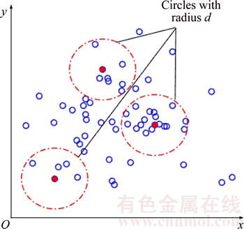
Figure 1 Illustration of local density model definition

The selection of radius is the most important step in computing the local density. The radius is most related to the property of the hyperspectral data, such as the number of the object classes, data range and data type. When the radius is chosen, there are two situations which will cause a detrimental effect. On the one hand, if radius is chosen too large, background pixels and anomalous pixels will be contained in the hypersphere together. Then, the local densities of all the pixels are big and similar. On the other hand, if radius is chosen too small, it will be over classified. In other words, the local densities of all the pixels are small and close to each other. The previous work in Ref. [19] utilizes the trial-and- error to obtain an appropriate radius. However, it needs priori knowledge about the dataset and costs more time in experiment. Thus, an adaptive method is employed by calculating the mean median of the distance matrix.

Owing to adopting a sliding dual-window, the assumption that most outer-region pixels belong to one class can be built. Then, the radius can be chosen as the mean median of the distance matrix.

Firstly, the distance matrix is computed as follows:

  (9)

where x_i is an outer-region pixel; dt_ij is the Euclidean distance between x_i and x_j; dt_i is the distance vector of the ith outer-region pixel to other outer-region pixels; D is the distance matrix.

Then, the medians for each column of D are obtained:

           (10)

Finally, the radius is chosen as

                             (11)

Equation (11) could guarantee that the radius is smaller than the distance between the background class and the anomalous class. Besides, the background pixels will have larger local densities than the anomalous pixels.

Figure 2 shows an ideal effect of the local density model. The data are selected from the HSI of Salinas Valley in Southern California [23]. It contains 150 grapes pixels, 9 lettuce pixels and 4 fallow pixels. Grapes are considered as background. The last two classes are considered as anomalies. From Figure 2, we can see that the local densities of grapes pixels are bigger than 100, while the local densities of lettuce and fallow pixels are smaller than 10. Thus, there is an obvious difference between background and anomalies.

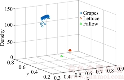
Figure 2 Illustration of local density model effect

The surrounding spatial neighborhoods for each PUT y are also denoted by The local density of each pixel in X_s is computed as follows:

           (12)

3.2 A two-step segmentation strategy

In order to remove the anomalies from X_s robustly, a two-step segmentation strategy is employed.

In the first step, since anomalies are of low- probability in background, preliminary segmentation based on an anomalous ratio is implemented. In general, the anomalous ratio is not more than 10% [19], thus we assume that 80% pixels with the largest local densities are background pixels and the other 20% contain both background pixels and anomalous pixels:

            (13)

In the second step, Otsu method is employed to obtain a discrimination threshold. Otsu method is a widely used technique in image segmentation by maximizing the separability between background and anomalous targets. In other words, it is a method to solve two-class-segmentation problem by maximizing the between-class variance. Firstly, gray the den_s as

                (14)

where [ ] denotes that the entries in den_sg are rounded. Then, the gray level denoted by th which maximizes the between-class variance is sought as follows:

                  (15)

where ω₀ and μ₀ are the probability and the mean of the entries which are smaller than the gray level, respectively; ω₁ and μ₁ are the probability and the mean of the entries which are not smaller than the gray level, respectively; μ is the mean of den_sg. If there are many values returned, the mean values of them are regarded as the threshold. Next, the final threshold denoted by th_f is obtained by de-graying th. The pixels whose local densities are larger than th_f are judged as background:

(16)

3.3 Overall procedure of LRXD or CRD with BRMLD

The overall procedure of LRXD or CRD with the background refinement method based on the local density (BRMLD-LRXD or BRMLD-CRD) is given as follows:

Step 1: Input the HSI data Y.

Step 2: For each PUT y of Y, the local background matrix X_s is built based on a dual- window.

Step 3: As Eqs. (9) to (11) shown, the radius d is chosen as the mean median of the distance matrix D.

Step 4: The local density is computed for each pixel in X_s with Eq. (12).

Step 5: A two-step segmentation strategy is employed to update X_s with Eq. (16).

Step 6: LRXD or CRD is employed to obtain the anomalous measurement for y by Eq. (2) or (7) with the updated X_s.

Step 7: The pixels whose anomalous measurements are bigger than the prescribed threshold are detected as anomalies.

4 Experimental results and discussion

In this section, to investigate the performance of the BRMLD-LRXD and BRMLD-CRD, experiments were conducted on two real HSI data.

4.1 Hyperspectral data description

The HSI data were collected through the SpecTIR Hyperspectral Airborne Rochester Experiment (SHARE) [24] on July 29, 2010 by the ProSpecTIR-VS2 sensor. There are 360 bands ranging from 390 nm to 2450 nm with a 5 nm spectral resolution and the original data contain 3137×320 pixels with a 1 m space resolution. In this study, two subareas which contain 100×100 pixels (Figure 3) and 120×80 pixels (Figure 4) are selected for simulations, respectively. In the first area (SpecTIR1, Figure 3), there are some square fabrics placed as targets in different spatial sized 9, 4, and 0.25 m² as displayed in Figure 3(b). The total number of target pixels is 72. In the second area (SpecTIR2, Figure 4), both of the four vehicles and two road signs were placed as targets. The groundtruth map includes 62 anomalous pixels corresponding to the 6 targets.

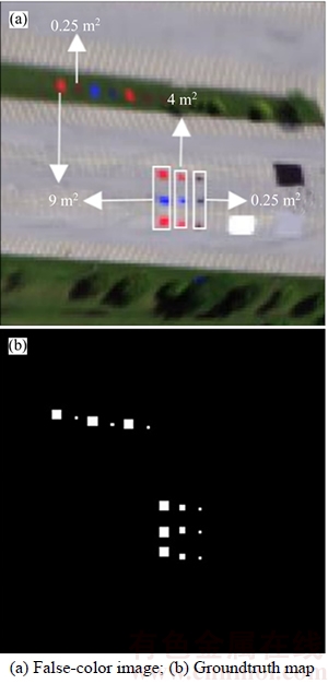
Figure 3 First area of SpecTIR hyperspectral data:

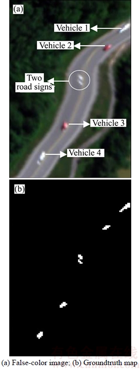
Figure 4 Second area of SpecTIR hyperspectral data:

4.2 Detection performance

In this section, BRMLD-LRXD and BRMLD- CRD are compared with LRXD, BACON, RSAD, PAD and CRD to evaluate the detection performance. For CRD, the detection performance is insensitive to the regularization parameter η [15]; hence, it is fixed to 1 in our experiments.

The detection performance of LRXD, CRD, BRMLD-LRXD and BRMLD-CRD is related with the size of the dual-window. Thus, in this work, w_in is chosen as 3, 5 and 7, and w_out is chosen as 11, 13 and 15. The receiver operating characteristic (ROC) [25] curves are employed as one of evaluation criteria. The probability of detection (P_d) and the probability of false alarm (P_f) are defined as

(17)

The area under the curve, referred to AUC, employed as other evaluation criteria in this experiment, which could reasonably estimate the accuracy of anomaly detection in respect of ROC analysis. A larger AUC represents higher anomaly detection accuracy.

Tables 1 and 2 give the AUC performance of LRXD, CRD, BRMLD-LRXD and BRMLD-CRD with varying window size for the two HSI data. Both tables show that BRMLD improves the detection performance of LRXD and CRD. For the SpecTIR1 data, Table 1 reveals that the best AUC performance of the four detectors can be achieved when the window sizes are set to (7, 11), (5, 11), (3, 15) and (3, 11) respectively. For the SpecTIR2 data, Table 2 illustrates that the best AUC performance of the four detectors can be achieved when the window sizes are respectively set to (7, 11), (7, 11), (7, 13) and (5, 15).

Table 1 AUC performance of LRXD, BRMLD-RXD, CRD and BRMLD-CRD with window size (w_in, w_out) for SpecTIR1 data

Table 2 AUC performance of LRXD, BRMLD-LRXD, CRD and BRMLD-CRD with window size (w_in, w_out) for SpecTIR2 data

The residuals between the best AUC and the worst AUC of the four detectors for the two HSI data are given in Table 3. The detectors with BRMLD have smaller residuals than the original detectors. It is clear that BRMLD can weaken the influence resulting from window size.

Table 3 Residuals between the best AUC and the worst AUC of LRXD, BRMLD-RXD, CRD and BRMLD- CRD

Figures 5 and 6 illustrate the ROC curves of all seven detectors for the two HSI data. The ROC curves of LRXD, CRD, BRMLD-LRXD and BRMLD-CRD are corresponding to their best AUC. For the SpecTIR1 data in Figure 5, BRMLD-LRXD and BRMLD-CRD obtain better detection performance than other five detectors. They achieve 1 probability of detection with a lower false alarm rate. Further, BRMLD-CRD achieves a higher detection probability than BRMLD-LRXD when the false alarm rate is lower than 0.02. After that, BRMLD-CRD begins to perform worse than BRMLD- LRXD, and its false alarm rate is slightly higher than BRMLD-LRXD when achieving 1 probability of detection.

Figure 5 ROC curves of LRXD, BACON, RSAD, PAD, CRD, BRMLD-LRXD and BRMLD-CRD for SpecTIR1 data

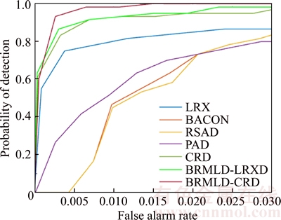
Figure 6 ROC curves of LRXD, BACON, RSAD, PAD, CRD, BRMLD-LRXD and BRMLD-CRD for SpecTIR2 data

For the SpecTIR2 data in Figure 6, we can find that BRMLD-LRXD and BRMLD-CRD outperform other five detectors throughout the curves. Compared with BRMLD-LRXD, BRMLD- CRD exhibits a slightly lower detection probability for a high false alarm rate (e.g., when the false alarm is 0–0.002). But, the overall detection performance of BRMLD-CRD is still better. On the other hand, BACON, RSAD and PAD perform worse than other four detectors with the higher false alarm rate when achieving 1 probability of detection.

In order to show the detail of the detection results, the three-dimensional plots of detection results from all seven detectors on the two HSI data are presented in Figures 7 and 8.

It can be seen that BACON, RSAD and PAD obtain larger values for the pixels which belong to the river in the southeast corner for the SpecTIR2 data. This is because BACON, RSAD and PAD implement detection based on global background assumption, in which some low-probability pixels probably could be detected as anomalies, while such pixels may be high-probability shown as background in local background assumption. In contrast, benefiting from the local detection strategy, LRXD, CRD, BRMLD-LRXD and BRMLD-CRD can detect the river pixels with small measurements.

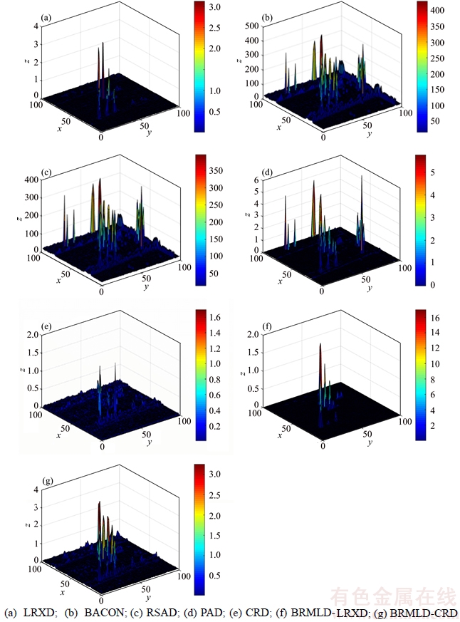
Figure 7 Plots of three-dimension detection results from seven different detectors on SpecTIR1 data:

For both data, compared with the basic detectors, BRMLD augments the detection results of anomalies while keeps the background pixels into a small range of values. From the above observations, the separability performance of BRMLD-LRXD and BRMLD-CRD are better than other detectors.

5 Conclusions

In this work, a background refinement method based on the local density is proposed for hyperspectral anomaly detection. Different from the previous parametric background refinement methods, BRMLD is nonparametric, and hence can be widely applied to different types of anomaly detectors. Anomalies among the background are removed based on calculating pixels’ local densities. This is followed by a two-step segmentation strategy which is designed to robustly remove the anomalies. Through BRMLD, a pure background is obtained. It strengthens the difference between background and anomalies. The experimental results for the two real HIS data indicate that BRMLD improves the detection performance and makes detection performance more stable.

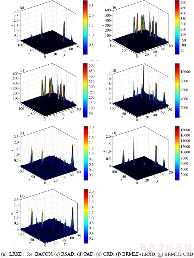
Figure 8 Plots of three-dimension detection results from seven different detectors on SpecTIR2 data:

References

[1] MANOLAKIS D, SHAW G. Clutter detection algorithms for airborne pulse-Doppler radar [J]. IEEE Signal Processing Magazine, 2010, 19(1): 29–43. DOI: 10.1109/SIU.2010. 5654379.

[2] BAJORSKI P. Target detection under misspecified models in hyperspectral images [J]. IEEE Journal of Selected Topics in Applied Earth Observations & Remote Sensing, 2012, 5(2): 470–477. DOI: 10.1109/JSTARS. 2012.2188095.

[3] ZHAO Chun-Hui, LI Jie, MEI Feng, et al. A kernel weighted RX algorithm for anomaly detection in hyperspectral imagery [J]. Journal of Infrared and Millim Waves, 2010, 29(5): 378–382. (in Chinese)

[4] STEIN D W J, BEAVEN S G, HOFF L E, et al. Anomaly detection from hyperspectral imagery [J]. IEEE Signal Processing Magazine, 2002, 19(1): 58–69. DOI: 10.1109/ 79.974730.

[5] ZHAO Chun-hui, WANG Yu-lei, LI Xiao-hui. A real-time anomaly detection algorithm for hyperspectral imagery based on causal processing [J]. Journal of Infrared Millim Waves, 2015, 34(1): 114–121. (in Chinese)

[6] CHANG C I, CHIANG S S. Anomaly detection and classification for hyperspectral imagery [J]. IEEE Transactions on Geoscience & Remote Sensing, 2002, 40(6): 1314–1325. DOI: 10.1109/TGRS. 2002.800280.

[7] ROBEY F C, FUHRMANN D R, KELLY E J, et al. A CFAR adaptive matched filter detector [J]. IEEE Transactions on Aerospace & Electronic Systems, 1992, 28(1): 208–216. DOI: 10.1109/7.135446.

[8] REN H, DU Q, CHANG C I, et al. Comparison between constrained energy minimization based approaches for hyperspectral imagery [C]// IEEE Workshop on Advances in Techniques for Analysis of Remotely Sensed Data (IEEE 2003). Greenbelt, USA: IEEE, 2003: 244–248. DOI: 10.1109/WARSD.2003. 1295199.

[9] CHEN Y, NASRABADI N M, TRAN T D. Simultaneous joint sparsity model for target detection in hyperspectral imagery [J]. IEEE Geoscience & Remote Sensing Letters, 2011, 8(4): 676–680. DOI: 10.1109/LGRS.2010.2099640.

[10] REED I S, YU X. Adaptive multiple-band CFAR detection of an optical pattern with unknown spectral distribution [J]. IEEE Transactions on Acoustics, Speech and Signal Processing, 1990, 38(10): 1760–1770. DOI: 10.1109/ 29.60107.

[11] KWON H, NASRABADI N M. Kernel RX-Algorithm: A nonlinear anomaly detector for hyper-spectral imagery [J]. IEEE Transactions on Geoscience & Remote Sensing, 2005, 43(2): 388–397. DOI: 10.1109/aero.2005.1559493.

[12] BANERJEE A, BURLINA P, DIEHL C. A support vector method for anomaly detection in hyperspectral imagery [J]. IEEE Transactions on Geoscience & Remote Sensing, 2006, 44(8): 2282–2291. DOI: 10.1109/tgrs.2006.873019.

[13] KHAZAI S, HOMAYOUNI S, SAFARI A, et al. Anomaly detection in hyperspectral images based on an adaptive support vector method [J]. IEEE Geoscience & Remote Sensing Letters, 2011, 8(4): 646–650. DOI: 10.1109/lgrs.2010. 2098842.

[14] SAKLA W, CHAN A, JI J, et al. An SVDD-based algorithm for target detection in hyperspectral imagery [J]. IEEE Geoscience & Remote Sensing Letters, 2011, 8(2): 384–388. DOI: 10.1109/ lgrs.2010.2078795.

[15] LI Wei, DU Q. Collaborative representation for hyperspectral anomaly detection [J]. IEEE Transactions on Geoscience & Remote Sensing, 2015, 53(3): 1463–1474. DOI: 10.1109/tgrs. 2014.2343955.

[16] BILLOR N, HADI A S, VELLEMAN P F. BACON: blocked adaptive computationally efficient outlier nominators [J]. Computational Statistics & Data Analysis, 2000, 34(99): 279–298. DOI: 10.1016/s0167-9473(99) 00101-2.

[17] DU Bo, ZHANG Liang-pei. Random-selection-based anomaly detector for hyperspectral imagery [J]. IEEE Transactions on Geoscience & Remote Sensing, 2011, 49(5): 1578–1589. DOI: 10.1109/tgrs.2010.2081677.

[18] GAO Lian-ru, GUO Qian-dong, PLAZA A, et al. Probabilistic anomaly detector for remotely sensed hyperspectral data [J]. Journal of Applied Remote Sensing, 2014, 8(1): 083538. DOI: 10.1117/1.jrs.8.083538.

[19] LOU Chen, ZHAO Hui-jie. Local density-based anomaly detection in hyperspectral image [J]. Journal of Applied Remote Sensing, 2015, 9(1): 095070–095070. DOI: 10.1117/ 1.jrs.9.095070.

[20] MOLERO A J M, GARZON E M, GARCIA I, et al. Analysis and optimizations of global and local versions of the RX algorithm for anomaly detection in hyperspectral data [J]. IEEE Journal of Selected Topics in Applied Earth Observations & Remote Sensing, 2013, 6(2): 801–814. DOI: 10.1109/jstars.2013.2238609.

[21] LI Wei, DU Q. Unsupervised nearest regularized subspace for anomaly detection in hyperspectral imagery [C]// IEEE, Geoscience and Remote Sensing Symposium (IGARSS 2013). Melbourne, Australia, 2014: 1055–1058. DOI: 10.1109/igarss.2013.6721345.

[22] LI Wei, TRAMEL E W, PRASAD S, et al. Nearest regularized subspace for hyperspectral classification [J]. IEEE Transactions on Geoscience & Remote Sensing, 2014, 52(1): 477–489. DOI: 10.1109/pic.2015.7489804.

[23] PLAZA A, MARTINEZ P, PLAZA J, et al. Dimensionality reduction and classification of hyperspectral image data using sequences of extended morphological transformations [J]. IEEE Transactions on Geoscience & Remote Sensing, 2005, 43(3): 466–479. DOI: 10.1109/tgrs.2004.841417.

[24] HERWEG J A, KEREKES J P, WEATHERBEE O, et al. Algorithms and technologies for multispectral, hyperspectral, and ultraspectral imagery XVIII (SPIE 2012) [C]// SHEN S S, ed. SPIE Proceedings: SPIE. 2012: 839028. DOI: 10.1117/12.919268.

[25] MOLERO A J M, GARZON E M, GARCIA I, et al. Anomaly detection based on a parallel kernel RX algorithm for multicore platforms [J]. Journal of Applied Remote Sensing, 2012, 6(1): 623–632. DOI: 10.1117/1.jrs.6.061503.

(Edited by YANG Hua)

中文导读

一种基于局部密度的高光谱异常检测背景纯化方法

摘要：在高光谱异常检测的基于背景的估计的研究中，背景中存在的异常像元会对背景估计的准确性产生不利影响，通过获得一个不包含异常目标的纯净背景可以有助于提高异常目标检测算法的检测率。因此，本文提出一种基于局部密度的背景纯化方法以去除背景中的异常像元。

经典的RX算法 (Reed-Xiaoli detector，RXD) 在背景统计信息估计时，因初始背景中存在异常像元而产生失真现象。这使RX算法的检测结果具有较高的虚警率。在本文中，将像元的局部密度作为该像元的异常度标签，通过最大类间方差法去除初始背景中潜在的异常像元，最后可以得到更纯净的背景集。利用纯化背景得到更准确的背景统计信息，可以有效降低RX算法的虚警率。

首先，通过度量一定半径内的光谱邻域，获得像元的局部密度，半径选取为距离矩阵的平均中位数；然后，基于局部密度设计了两步分割策略：第一步，将原始背景分割为一个包含大部分背景像元的集合及一个混合着背景像元和异常像元的小子集。第二步，利用最大类间方差法处理小子集，获得一个判别阈值，去除局部密度小于该阈值的像元，得到纯净的背景。最后，利用RX检测算法和基于协同表示的检测算法验证所提背景纯化算法的有效性。

本文算法对于圣地亚哥海军基地数据和SpecTIR数据，AUC值比LRXD分别提高了0.0246和0.0068，并且相比于其它算法有较高的检测率。实验结果说明，密度背景纯化方法有效抑制了异常点对背景数据的干扰，使背景协方差和均值等参数更准确，降低了虚警率。在计算密度时，需要人为设定半径值。对于两幅高光谱数据，在不同半径选择下DBRAD最大AUC差值为0.0088和0.0012，实验结果表明，人为选择半径值可能会对最后的检测效果造成较大影响。如何自适应选取半径将是下一步研究的重点。

关键词：高光谱图像；异常检测；背景纯化；局部密度

Foundation item: Projects(61405041, 61571145) supported by the National Natural Science Foundation of China; Project(ZD201216) supported by the Key Program of Heilongjiang Natural Science Foundation, China; Project(RC2013XK009003) supported by Program Excellent Academic Leaders of Harbin, China; Project(HEUCF1508) supported by the Fundamental Research Funds for the Central Universities, China

Received date: 2016-04-21; Accepted date: 2017-12-01

Corresponding author: ZHAO Chun-hui, Professor; E-mail: zhaochunhui@hrbeu.edu.cn; ORCID: 0000-0002-8015-387X

Abstract: For anomaly detection, anomalies existing in the background will affect the detection performance. Accordingly, a background refinement method based on the local density is proposed to remove the anomalies from the background. In this work, the local density is measured by its spectral neighbors through a certain radius which is obtained by calculating the mean median of the distance matrix. Further, a two-step segmentation strategy is designed. The first segmentation step divides the original background into two subsets, a large subset composed by background pixels and a small subset containing both background pixels and anomalies. The second segmentation step employing Otsu method with an aim to obtain a discrimination threshold is conducted on the small subset. Then the pixels whose local densities are lower than the threshold are removed. Finally, to validate the effectiveness of the proposed method, it combines Reed-Xiaoli detector and collaborative-representation-based detector to detect anomalies. Experiments are conducted on two real hyperspectral datasets. Results show that the proposed method achieves better detection performance.