
Trans. Nonferrous Met. Soc. China 24(2014) 509-513
Three-dimensional magnetotelluric regularized inversion based on smoothness-constrained model
Xiao-zhong TONG1,2, Jian-xin LIU1, Rong-wen GUO1, Hai-fei LIU1, Lu GONG1
1. School of Geosciences and Info-physics, Central South University, Changsha 410083, China;
2. Key Laboratory of Nonferrous Resource and Geological Hazard Detection of Hunan Province, Central South University, Changsha 410083, China
Received 30 December 2012; accepted 27 April 2013
Abstract:
How to get the rapid and stable inversion results and reconstruct the clear subsurface resistivity structures is a focus problem in current magnetotelluric inversion. A stable solution of an ill-posed inverse problem was obtained by the regularization methods in which some desired structures were imposed to stabilize the inverse problem. By the smoothness-constrained model and approximate sensitivity method, the stable subsurface resistivity structures were reconstructed. The synthetic examples show that the smoothness-constrained regularized inversion method is effective and can be reasonable to reconstruct three-dimensional subsurface resistivity structures.
Key words:
magnetotelluric; regularized inversion; approximate sensitivity; smoothness-constrained model;
1 Introduction
To invert magnetotelluric data for three-dimensional electrical conductivity structures has been a major challenge in applied geophysics for many years. Three-dimensional inversion involves forward modelings for general three-dimensional structures, which is very computationally time-consuming compared with the one-dimensional and two-dimensional inverse problems. Despite this difficulty, several attempts have been made to carry three-dimensional inversions using different forward numerical solutions. MACKIE and MADDEN [1] developed an inversion procedure for magnetotelluric data based on the finite difference and conjugate gradient methods. ZHDANOV and TOLSTAYA [2] used the integral equation to formulate three-dimensional magnetotelluric inverse problems with a minimum support nonlinear parameterization in the solution. NEWMAN [3] presented an inversion scheme in which the finite difference method is used for the forward modeling and the integral equation for the inverse formulation. HAN et al [4] used the finite element method and approximate sensitivities to formulate three-dimensional magnetotelluric inverse problems. These inversion methods required powerful higher-end workstations or supercomputers. Thus, it is commonly accepted that three-dimensional magnetotelluric inversions are too expensive and cannot be a practical interpretation tool for most field geophysicists.
Large-scale inverse problems are usually underdetermined, meaning that there are more unknowns, typical in the forms of highly digitized model meshes. A stable solution of an ill-posed inverse problem can be obtained by the regularization methods [5-7] in the objective functional subjected to a minimum. The regularization is to search for a solution within a specific class of selected models. The traditional way to implement regularization in inverse problem solutions is to select the class of inverse models with a smooth distribution of model parameters.
The main difference between the present inversion method and those previous works is that the present smoothness-constrained inversion approach is applied to solving the three-dimensional magnetotelluric data. Firstly, the modeling code was concludes which used the finite element method and was designed to deal with the three-dimensional forward problem. In order to check the validity of the code, the numerical results were compared with the analytical solutions. Secondly, a smoothness-constrained least-squares inversion method was developed to describe the adjoint-equation method for calculating the sensitivities. Finally, the inversion method was tested on synthetic data to verify its performance.
2 Forward modeling
2.1 Governing equation
At the low frequency used in magnetotelluric, displacement currents are negligible and there is no electric current source in magnetotelluric problems. Assuming a time harmonic dependence of  , the pair of vector equations can be expressed as
 (1)
(1)
 (2)
(2)
where E and H are the electric and magnetic fields, respectively; �� is the angular frequency; �� is the spatially variable electrical conductivity; �� (��=4p��10-7 H/m) is the magnetic permeability of free space. No finite source is considered in the above equations because a plane-wave source is assumed in the magnetotelluric method. From Eqs. (1) and (2), the governing equation of the electric field, E, can be obtained as
 (3)
(3)
2.2 Finite element equation
To solve the governing differential Eq. (3) by the finite element method, firstly, a computing domain into is divided non-uniform grid capable of modeling irregular geometries, as shown in Fig. 1. Then utilizing the finite element method, the linear system can be derived as follows [8]:
KE=p (4)
where K is a large sparse, banded, symmetric, ill-conditioned, non-Hermitian complex matrix, and p is the source vector that depends on the boundary conditions and source field polarization. This system can be efficiently solved using the Bi-CGSTAB method [9], which belongs to the class of Krylov subspace techniques that are highly efficient in iteratively solving sparse linear system. Considering boundary conditions, the electric field of each point can be obtained by solving linear equation.
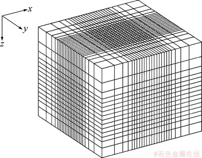
Fig. 1 Non-grid imposed upon the earth model to simulate three-dimensional magnetotelluric fields
2.3 Verification of forward solution
To test the forward modeling algorithm, the code is applied to a homogeneous half-space. For a nonmagnetic homogeneous half-space, the analytical response can be expressed as [10]
 (5)
(5)
where  is the electric field on the earth��s surface.
Considering a homogeneous half-space of 100 ����m, the numerical solutions computed by the finite element method (FEM) and the analytical solutions on the surface are shown in Fig. 2. The finite element method responses are in good agreement with the analytical responses.
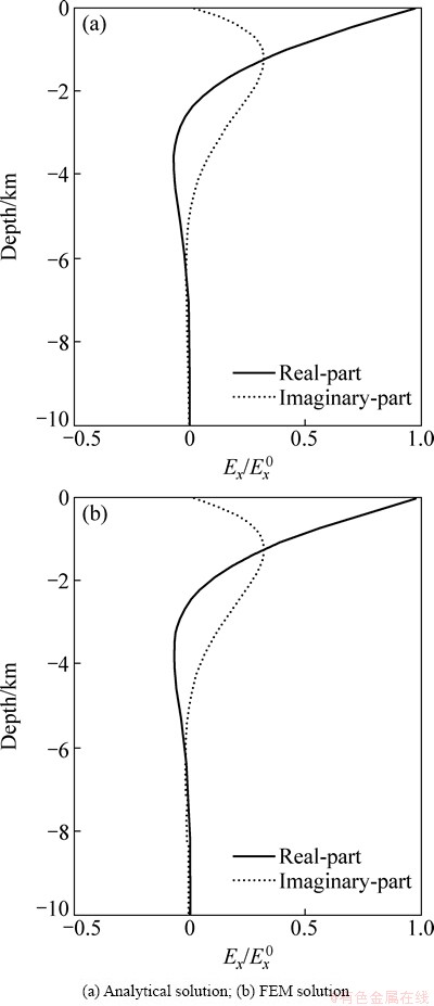
Fig. 2 Magnetotelluric response of 1 Hz on surface of a 100 ����m half-space
From this result, it is confirmed that the forward modeling method is effective.
3 Inverse problem
3.1 Smoothness-constrained least-squares method
Inverse problem of magnetotelluric sounding data is ill-posed and non-linear, and can be solved by some regularization methods. The following parametric functional is minimized in the regularization [5].
 (6)
(6)
where  is a misfit function, S(m) is a stabilizing function, �� is a regularization parameter which controls the trade-off between these two contributions in this minimization process. The misfit and stabilizing functions are written as
 (7)
(7)
 (8)
(8)
where F is a forward modeling operator which is generally non-linear, m is a model parameter vector, d is a model response (predicted data) vector, and C indicates the model parameter weighting matrix [11].
There have been many algorithms suggested so far to solve Eq. (6) [12,13]. In this work, the smoothness-constrained least-squares inversion is adopted for solving the regularized inverse problems. Linearization of Eq. (6) and some manipulation yields:
 (9)
(9)
where ��d is the error or discrepancy vector between the observed and calculated data, ��m denotes the model updates to be obtained, J is the sensitivity matrix or Jacobian matrix of forward modeling operator F, and C is a Laplacian (second-order) smoothness operator.
3.2 Sensitivity calculation
In principle, the sensitivities can be computed by three methods: the brute-force method, the sensitivity- equation method, and the adjoint-equation method [14]. The computation times of these methods are roughly equal to N��Mf, N��Mf and Mo��Mf forward computations respectively (N is the number of model parameters, Mf is the number of frequencies and Mo is the number of observation locations). Because there are more model parameters than observations on inversion, the adjoint-equation method is therefore the most efficient method in calculating the sensitivities.
We have used the adjoint-equation method for the calculation of the sensitivities, which is used by FARQUHARSON and OLDENBURG [15] for electromagnetic inverse problem. For the purposes of the inversion, the conductivity is represented as a finite linear combination of suitable basis functions:
 (10)
(10)
where ��j are the basis functions and ��j are the coefficients.
The sensitivity with respect to the conductivity of the j th cell can be given by
 (11)
(11)
where the auxiliary field, E��, is defined as the electric field in the domain, f is any component of the electric or magnetic field, and vj is the volume of the jth cell.
3.3 Determination of regularization parameters
Determination of the regularization parameter (Lagrangian multiplier), which balances the minimization of the data misfit and model roughness, may be a critical procedure to achieve both resolution and stability. In our implementation, the adaptive regularization parameter algorithm is adopted [16], which is defined as
 (12)
(12)
where k is the kth iteration. Just as for the implementations of the discrepancy principle and the adaptive approach, the regularization parameter is chosen at the kth iteration according to the expression:
 (13)
(13)
where 0.01��c��0.5, and ��* is the minimizer of the adaptive algorithm given in Eq. (12).
4 Examples for synthetic data
4.1 Two-dimensional model
The two-dimensional model used to generate the data is shown in Fig. 3. It consists of a 0.5 ����m conductive block with dimensions of 1 km��2 km in a 100 ����m background half-space. The top of the conductive block is at a depth of 250 m, and its bottom is at a depth of 2250 m beneath of the surface.
For numerical forward modeling, the two- dimensional model, 6 km��6 km��3 km, was unevenly discretized into 54��54��44 cells, including the 10 km air layer. Magnetotelluric data from a total of 81 magnetotelluric soundings are used in the inversion, and the magnetotelluric frequencies used here range from 0.1 to 120 Hz. The inversion takes six iterations to reduce the misfit to 0.093, and the inversion results are shown in Fig. 4. From the inversion result, a low resistivity can be clearly identified anomaly in the inverted section. It is clear that the smoothness-constrained inversion algorithm for magnetotelluric data can effectively recover the simple geo-electrical model.
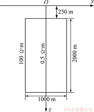
Fig. 3 Two-dimensional model used to generate magneto- telluric data
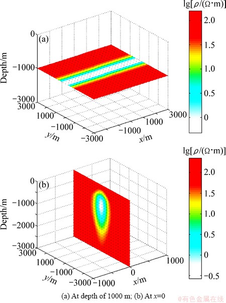
Fig. 4 Slices for two-dimensional model of three-dimensional inversion
4.2 Three-dimensional model
The three-dimensional model used to generate the data is shown in Fig. 5. It consists of a 0.5 ����m buried body with size of 1 km��2 km��2 km in a 100 ����m background half-space. The top of the buried body is at a depth of 250 m, and its bottom is at a depth of 2250 m beneath of the surface.
For numerical forward modeling, the three- dimensional model, 6 km��6 km��3 km, is unevenly discretized into 54��54��44 cells, including the 10 km air layer. Magnetotelluric data from a total of 81 magnetotelluric soundings are used in the inversion, and the magnetotelluric frequencies used here range from 0.1 to 120 Hz. The inversion takes six iterations to reduce the misfit to 0.128, and the inversion results are shown in Fig. 6. From the above model study, it is confirmed that the smoothness-constrained inversion of magnetotelluric data can efficiently reconstruct three-dimensional subsurface resistivity structures.
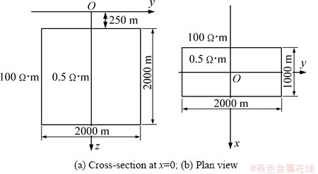
Fig. 5 Three-dimensional model used to generate magneto- telluric data
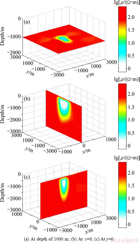
Fig. 6 Different horizontal and vertical depth slices for model of three-dimensional inversion
5 Conclusions
1) A regularized method to invert the magnetotelluric data of three-dimensional structures was developed, with the forward calculations based on the finite element method. The system of equations resulted from the finite-element was solved by the iterative Bi-CGSTAB method, which is a Krylov subspace technique with high efficiency in solving sparse linear system.
2) The sensitivities were obtained from the adjoint-equation method, which is among the most efficient methods of calculating the sensitivities. The inverse problem was formulated to have a smooth structure and incorporate a desired reference model, which was solved by an iterative lease-squares method.
3) The synthetic examples showed that three- dimensional inversions are effective and give reasonably accurate results for simple three-dimensional problems. However, as more complicated problems or field data are considered, further work should be required.
References
[1] MACKIE R L, MADDEN T R. Three-dimensional magnetotelluric inversion using conjugate gradients [J]. Geophysical Journal International, 1993, 115(1): 215-229.
[2] ZHDANOV M, TOLSTAYA E. Minimum support nonlinear parametrization in the solution of a 3D magnetotelluric inverse problem [J]. Inverse Problem, 2004, 20(6): 937-952.
[3] NEWMAN G A. Crosswell electromagnetic inversion using integral and differential equations [J]. Geophysics, 1995, 60(3): 899-911.
[4] HAN N, NAM M J, KIM H J. Efficient three-dimensional inversion of magnetotelluric data using approximate sensitivities [J]. Geophysical Journal International, 2008, 175(2): 477-485.
[5] TIKHONOV A N, ARSENIN V Y. Solution of ill-posed problems [M]. New York: Wiley, 1977.
[6] FARQUHARSON C G, OLDENBURG D W. A comparison of automatic techniques for estimating the regularization parameter in non-linear inverse problems [J]. Geophysical Journal International, 2004, 156(3): 41-425.
[7] LI Ai-yong, CAO Chuang-hua, LIU Jian-xin. Effects of different amplitudes of noise and missing data on regular inversion of magnetotelluric response [J]. The Chinese Journal of Nonferrous Metals, 2012, 22(3): 915-921. (in Chinese)
[8] TONG Xiao-zhong, LIU Jian-xin, XIE Wei, XU Lin-hua, GUO Rong-wen, CHENG Yun-tao. Three-dimensional forward modeling for magnetotelluric sounding by finite element method [J]. Journal of Central South University of Technology, 2009, 16(1): 136-142.
[9] SMITH J T. Conservative modeling of 3-D electromagnetic fields. Part ��: Biconjugate gradient solution and an accelerator [J]. Geophysics, 1996, 61(5)��1319-1324.
[10] LIU Jian-xin, TONG Xiao-zhong, RONG Rong-wen. Magnetotelluric sounding methods exploration [M]. Beijing: Science Press, 2012. (in Chinese)
[11] de GROOT-HEDLIN C, CONSTABLE S. Occam��s inversion to generate smooth, two-dimensional models from magnetotelluric data [J]. Geophysics, 1990, 55(12): 1613-1624.
[12] CANDANSAYAR M E. Two-dimensional inversion of magnetotelluric data with consecutive use of conjugate gradient and least-squares solution with singular value decomposition algorithms [J]. Geophysical Prospecting, 2008, 56(1): 141-157.
[13] KERRY K. 1D inversion of multicomponent, multifrequency marine CSEM data: Methodology and synthetic studies for resolving thin resistive layers [J]. Geophysics, 2009, 74(2): F9-F20.
[14] McGILLIVRAY P R, OLDENBURG D W. Methods for calculating Fr��chet derivatives and sensitivities for the non-linear inverse problem: a comparative study [J]. Geophysical Prospecting, 1990, 38(5): 499-524.
[15] FARQUHARSON C G, OLDENBURG D W. Approximate sensitivities for the electromagnetic inverse problem [J]. Geophysical Journal International, 1996, 126(1): 235-252.
[16] MAO Li-feng, WANG Xu-ben, CHEN Bin. Study on an adaptive regularized 1D inversion method of helicopter TEM data [J]. Progress in Geophysics, 2011, 26(1): 300-305. (in Chinese).
���ڹ⻬Լ��ģ�͵Ĵ�ص����ά������
ͯТ��1,2��������1��������1��������1���� ¶1
1. ���ϴ�ѧ �����ѧ����Ϣ����ѧԺ����ɳ 410083��
2. ���ϴ�ѧ ��ɫ��Դ������ֺ�̽�����ʡ�ص�ʵ���ң���ɳ 410083
ժ Ҫ����εõ������ȶ��ķ��ݽ�����������ؽ����µ����ʽṹ��������Ȼ�ǵ�ǰ��ص�ŷ����о���һ���ص㡣�ڹ���Ŀ�꺯���в�����������ʹ���ʶ�������������ȶ��ķ��ݽ���������ƽ���ȶ��Ժͷ�Ψһ�ԣ����⻬Լ��ģ�ͺͽ��������Ⱦ�����ⷽ��Ӧ���ڷ��ݹ����У������ȶ��ع������µ����ʽṹ������ģ������Ľ�������⻬Լ�������ݷ����ǿ��еģ����ܺ������ؽ�������ά�����ʽṹ��
�ؼ��ʣ���ص�ţ������ݣ����������Ⱦ��⻬Լ��ģ��
(Edited by Hua YANG)
Foundation item: Project (20110162120064) supported by Higher School Doctor Subject Special Scientific Research Foundation of China; Project (10JJ6059) supported by the Natural Science Foundation of Hunan Province, China
Corresponding author: Xiao-zhong TONG; Tel: +86-731-88877075; E-mail: csumaysnow@csu.edu.cn
DOI: 10.1016/S1003-6326(14)63089-2
Abstract: How to get the rapid and stable inversion results and reconstruct the clear subsurface resistivity structures is a focus problem in current magnetotelluric inversion. A stable solution of an ill-posed inverse problem was obtained by the regularization methods in which some desired structures were imposed to stabilize the inverse problem. By the smoothness-constrained model and approximate sensitivity method, the stable subsurface resistivity structures were reconstructed. The synthetic examples show that the smoothness-constrained regularized inversion method is effective and can be reasonable to reconstruct three-dimensional subsurface resistivity structures.
