
J. Cent. South Univ. (2012) 19: 206-212
DOI: 10.1007/s11771-012-0993-6![]()
Traffic condition estimation with pre-selection space time model
DONG Hong-hui(�����), SUN Xiao-liang(������), JIA Li-min(������),
LI Hai-jian(���), QIN Yong(����)
State Key Laboratory of Rail Traffic Control and Safety, Beijing Jiaotong University, Beijing 100044, China
? Central South University Press and Springer-Verlag Berlin Heidelberg 2012
Abstract:
A pre-selection space time model was proposed to estimate the traffic condition at poor-data-detector, especially non-detector locations. The space time model is better to integrate the spatial and temporal information comprehensibly. Firstly, the influencing factors of the ��cause nodes�� were studied, and then the pre-selection ��cause nodes�� procedure which utilizes the Pearson correlation coefficient to evaluate the relevancy of the traffic data was introduced. Finally, only the most relevant data were collected to compose the space time model. The experimental results with the actual data demonstrate that the model performs better than other three models.
Key words:
traffic condition; estimation; space time model; pre-selection��
1 Introduction
In the past decade, as the traffic jam has been increasing in many cities, many advanced transportation technologies and systems have been proposed to relieve the congestion. One of the major elements in these technologies is traffic condition estimation and prediction. Traffic control and management systems as well as traffic information guidance systems can all benefit from accurate and implementable traffic condition estimation and prediction techniques.
However, due to the huge road segments and intersections of urban road network and the constraint of government investment funds, it is incapable to install detectors everywhere. It is hard to access complete traffic information covering the whole network, especially at non-detection locations [1]. In addition, missing or corrupted detector data are unavoidable in practice. In order to obtain the accurate, timely and complete traffic information, it becomes more and more important to develop an effective method to estimate the traffic condition at the poor-data-detector, especially the non-detector locations.
There have been amounts of works on the subject of traffic condition estimation and prediction. Many prediction models including historical average model, linear models, time series model, Kalman filtering, and so on, are used in this subject. In particular, time series model is used frequently and developed using techniques such as autoregressive integrated moving average (ARIMA), nonparametric regression, neural networks, etc [2-5]. However, these models are mostly based on the state-space methodology and rarely consider the spatial correlation in traffic system [6].
Researches on the traffic condition estimation at non-detection locations also exist. The methods such as historical average method, principal component method, stepwise regression method, correlation analysis, gray neural network and cluster analysis are used in this filed [7]. Most of these methods applied the classical forecasting to the project of traffic condition at non- detector locations. However, the low accuracy and lack of application are unable to meet the traffic information demands [1].
Recent researches have shown the importance of spatial correlation in traffic systems. The space-time model is better to account for the spatial correlation and is well suited for the applications of large spatial scale. Meanwhile, the model can integrate the spatial and temporal information simultaneously to predict the traffic condition [8]. KAMARIANAKIS and PRASIACOS [9] applied a space-time autoregressive integrated moving average (STARIMA) model to predicting the traffic flow parameters. Their model assumes that the spatial correlations are adjacency-based weights considering the topology only. MIN et al [10] developed a new spatial structure considering both the travel speed and distance under different road types and traffic conditions. Meanwhile, they assumed the weight is nonzero only if one can travel through during the given time, and their models achieve a good result. However, using all the related segments as input variables would involve much irrelevance and redundancy, and would be prohibitive for computation [11]. Thus, an effective method to reduce the estimated parameters is urged.
The focus of this work is to explore a space-time model to estimate the traffic condition at the poor-data-detector locations, especially the non-detector locations. To induce the estimated parameters of traditional space-time model, a pre-selection ��cause nodes�� procedure is proposed to solve the problem. The ��cause nodes�� are defined as the most informative or critical variables to the target in the estimation process. This work firstly summarizes the influencing factors of the ��cause nodes��, and then chooses the candidate input data restricted in a certain road network based on the factors. Secondly, the Pearson correlation coefficient is used to evaluate the relevancy of the data to find the ��cause nodes��. Finally, the space time model based on the selected ��cause nodes�� can be constructed, which will make the model a good performance.
2 space time model
Traffic condition data analysis is a classic application of time series analyses, giving the seemingly random behavior of traffic. At the same time, traffic flow is generally constrained along a one-dimensional pathway (e.g. a travel lane), and the traffic condition at one pathway has some relationship with its neighbors due to the direction and continuity of the traffic flow. Hence, a space time estimation model provides a solution to integrate the spatial and temporal features, which is important to improve the accuracy and reliability of estimation model.
To illustrate the space time model, a situation can be visually represented by Fig. 1, where i-1, i and i+1 represent three neighboring sections; t-1, t and t+1 denote the different time. xi,t is the detector data representing the flow rate, velocity, and occupancy at time t on section i. In addition, the solid ellipses denote the sections equipped with detectors; the dashed ones denote non-detector section or poor-data-detector sections. The arrows denote the relationship between the detectors. As the vehicles move, xi,t not only depends on its past data xi,t-1, but also depends on the time series of its neighboring data such as {xi-1, t-1, xi-1, t} and {xi+1, t-1, xi+1, t}. That��s to say, xi,t can be estimated with the spatial and temporal information of its neighboring locations i-1, i+1 and its past data. This is the intuition of the present space-time estimation model.
Fig. 1 Typical space time model structure
Suppose the sections i-1, i-2, ��, i-c are the downstreams of section i, and the upstreams are sections i+1, i+2, ��, i+d, to estimate the traffic condition xi, t. It considers not only the downstream and upstream data of the current time, but also the past time series xi+j(t-k) (k= l, 2, ��, p, j=-c, -c+1, ��, -1, 1, 2, ��, d). The basic space-time estimation model is described as
![]()
![]()
![]() (1)
(1)
where f is an unknown function describing the relationship between the target section and its neighbors; e is the relative error.
A family of space-time models called space-time autoregressive moving average (STARMA) was first presented in the early 1980s by PFEIFER and DEUTSCH [12-13]. These models are characterized by auto-regressive and moving-average terms lagged both in space and time. Since then it has been applied to spatial time series data with a wide variety of disciplines such as river flow [12], spread of disease [13], and spatial econometrics [14]. KAMARIANAKIS et al [8-9] firstly used the STARMA model to predict traffic condition. It is believed that a similar approach can be carried out for non-detector traffic condition estimation.
However, in the parameters estimation process of the STARMA (p,q) model, there are almost T(p+q)N2 parameters to be calculated, where T is the time dimension, and N corresponds to the section number of the road network [10]. In this work, T=k and N=c+d. It is particularly difficult to estimate all the parameters for the large scale road network with huge section number. On the other side, the space time model using all the neighboring sections as input variables would involve much irrelevance, redundancy, and would be prohibitive for computation [11]. Consequently, an effective method to reduce the estimated variables and preselect the ��cause nodes�� procedure is of great demand.
3 Pre-selection procedure of cause nodes
In a transportation network, as the vehicles move, the traffic flow of the upstream or downstream may be informative to the target one. Thus, the traffic condition at the poor-data-detector or non-detector location using the adjacent traffic data can be estimated. There are a large number of adjacents, and it is much important to study the distribution law of the traffic data space and find a way to reduce the estimated numbers of the traditional space-time model to estimate the original traffic condition. To solve this problem, a method of ��cause nodes�� pre-selection procedure is proposed. The ��cause nodes�� are represented by the most relative variables (or values) to the target one, which will be effective enough to construct the space-time traffic condition estimation. Therefore, designing a good ��cause nodes�� selector is important to the success of the overall model.
Consequently, the influencing factors of the ��cause nodes�� are studied firstly.
3.1 Influencing factors of cause nodes
The most important issue to select the ��cause nodes�� is to define the correlation coefficient. The motivation is very intuitive. Stronger relationship serves more important in the traffic estimation model.
For simplicity and scalability, the Pearson correlation coefficient is used as the specific ranking. In statistics, the Pearson correlation coefficient (typically denoted by r) is a measure of the correlation (linear dependence) between two variables, X and Y, giving a value between +1 and -1. The coefficient can be estimated by
![]() (2)
(2)
where X is a set of n samples {xi}(i=1, ��, n); Y is a set of m samples {yi}(i=1, ��, m); ![]() is the mean arithmetical value of X and
is the mean arithmetical value of X and ![]() is the mean arithmetical value of Y. The following statements can be stated about the coefficient:
is the mean arithmetical value of Y. The following statements can be stated about the coefficient:
1) r>0 represents the positive correlation, while r<0 denotes the negative correlation.
2) |r|=1, if only X and Y are totally related.
3) |r|=0, if only X and Y are completely independent.
Except for the correlation coefficient, the distance is also important to measure the relationship. In the urban road network, there exist amounts of sensors (loop detectors, microwave detectors and video detectors) equipped on the road segments to detect and measure the traffic condition. However, a sensor can only give random behaviors of the place where it locates. In a certain distance away, due to the continuity and randomicity of traffic flow, the detected data may not represent the traffic condition well.
In Ref. [15], the 2nd Ring Road in Beijing was taken for example to test how far the detector data will be informative. The data are from April 14-18, 2008 collected from microwave detectors of the Beijing Expressway Traffic Information Detection System. Except for three faulty detectors, a total of 49 detectors were included. Figure 2(a) shows the study area and the detector locations. Figure 2(b) shows a coordinate system, where the vertical line represents the Pearson correlation coefficient between the volume and distance, and the horizontal line represents the distance. It is easy to find that the coefficient shrinks when the distance gets longer.
Fig. 2 Detector locations of 2nd Ring Road in Beijing (a) and correlation between traffic volume and distance (b) [18]
Apparently, not all the adjacent data are informative to the target one. The same conclusion are also appeared in Ref. [16]. In Ref. [16], the farthest upstream point is the detector (location) that a vehicle can start and still arrive at target location (detector) within a defining time period and at the designated maximum speed allowed for the section of roadway. The farthest downstream point is the detector (location) that a vehicle can travel from the target detector (location) within a giving time term and at a designated speed. As mentioned above, the distance is of great importance to the ��cause nodes�� selection.
Actually, the vehicles upstream will soon drive to downstream, and the direction will also affect on judging the relevancy of traffic flow. In Ref. [15], the coefficient between traffic volume and distance in Beijing was calculated. It is also noticed that the strongly correlated coefficient (relatively high correlation coefficient) with the object traffic flow is almost from upstream links. Meanwhile, it is also found that the correlation coefficients are different with different time lags.
Observably, the coefficients are dependent on the location of detectors, direction of traffic flow and time lags. The analysis above provides basis for ��cause nodes�� pre-selection procedure.
3.2 Flow chart of pre-selection procedure
Selecting the right sets (or features) is one of the most primary tasks of the ��cause nodes�� selector. Thus, it can be regarded as a variable and feature selection algorithm in the field of machine learning. Variable and feature selection is often an essential data processing step prior to applying a learning algorithm. It aims to seek optimal or suboptimal sets by preserving the main information carried by the collected complete data to facilitate future analysis for high dimensional problems [17].
Let S={x1, x2, ��, xn} be the collected full data set formed by a total of N observations (instances) and n attributes in the measurement space, where the k-th instance vector is {x1(k), x2(k), ��, xn(k)} and the observation vector for the j-th attribute is xj={xj(1), xj(2), ��, xj(N)}T. The objective of the selection is to find a subset Sd={z1, z2, ��, zd}=![]() which can be used to represent the original data S, where zm=
which can be used to represent the original data S, where zm=![]() im
im![]() {1, 2, ��, n}, m=1, 2, ��, d with d��n (generally d<
{1, 2, ��, n}, m=1, 2, ��, d with d��n (generally d<
xi=f(z1, z2, ��, zd)+e (3)
where f is an unknown function which should be estimated, and e is the relative error .
There exist some variables and feature selection algorithms, such as the nearest neighbor learner, decision tree algorithms, principal component analysis (PCA) and variable ranking. There are also some algorithms adopting correlation coefficient r as a variable ranking criterion because of its simplicity, scalability and goodness of linear fit for individual variables [17]. Usually, positively correlated variables are top ranked and negatively correlated variables are bottom ranked. In Ref. [11], their model chooses a number of candidate subsets randomly among the top ranked variables based on the Pearson correlation coefficient, and then combines those subsets through a fusion methodology to implement the traffic flow prediction. Though their model achieves a good performance, it is hard to determine the number of candidate sets objectively. The forward stepwise selection method is thus chosen.
Forward stepwise selection begins with independent variables being entered into the regression equation one at a time, and the provided predictors meet the statistical significance criteria with the dependent variable. Selection of independent variable entry will be based on the descending order of the largest significant correlation coefficient. Independent variables will enter into the regression until an independent variable does not uniquely influence the dependent variable. Assume that a variable subset Sd-1, consisting of d-1 significant variables, z1, z2, ��, zd-1, has been determined at step d-1, and the d-th significant feature zd will be chosen in such a manner: The subset Sd-1+{zd} should be the most ��representative�� and, thus, the most ��informative�� subset compared with any other subsets formed by adding a candidate feature zd to Sd-1.
The selection strategy used for ��cause nodes�� selection can be described as follows: 1) Collect the topology of the road network and collect all the available traffic data; 2) All detector data within a certain distance upstream of target site (detector location) will be used as the original input variables, and the distance depends on the time horizon and the designated speed limits. 3) The Pearson correlation coefficients are calculated between the data of target site and the input variables with different time lags, respectively. 4) The foreword stepwise regression is used to choose the most relevant data as the so-called ��cause nodes�� set Sd.
��Cause nodes�� selection procedure uses the Pearson correlation coefficient to calculate the relevancy of the traffic flow limited to a given area as the candidates, and then the candidates with the highest merit selected by foreword stepwise regression method are used to compose the space time estimation model for training and testing. The components of pre-selection ��cause nodes�� space time model are shown in Fig. 3.
The model proposed above is heavily dependent on the history traffic data in the training process. However, there is not enough historical data at the poor-data- detector, especially at the non-detector locations, which makes their relevancy hard to be calculated. Thereby, the data of the same traffic patterns are utilized instead.
Fig. 3 Components of pre-selection ��cause nodes�� space-time model
4 Data preparation
4.1 Study area and data source
Because of long-time employment or lack of maintenance of the detectors, missing or corrupted sensor data are unavoidable in practice. Meanwhile, there exist a large number of road segments and intersections without equipping detectors in Beijing. How to obtain the traffic condition of those sites should be considered. These are the main problems to be solved in this work.
To illustrate the application of the methodology to actual data, test road networks (shown in Fig. 4) selected from North 3rd Ring and North 4th Ring Road of Beijing are under consideration. The dots in Fig. 4 represent the detector locations numbered 1, 2, ��, 18; the link between two detectors is defined as a segment. There are 18 detectors and 17 segments in the test network in all, and the segments are all expressway links.
The data analyzed in this work were collected from the Expressway Traffic Information Detection System which covers nearly all the expressways including 2nd Ring Road, 3rd Ring Road, 4th Ring Road, 5th Ring Road and other 15 radiation expressways. The detector data include volume, average velocity, time occupancy and large car volume every 2 min. Such timing would be too short to be used for estimation. For this reason, the collected data are then transformed into discrete time series recorded during every 5 min.
4.2 Measures of performance
There are several summary statistics to evaluate the performance of the estimation model, including root mean square error (RMSE), mean absolute deviation (MAD), absolute percentage error (APE), and so on. Absolute percentage error provides the most useful basis for comparison as traffic flow observations vary from time to time. For this reason, the mean absolute percentage error (MAPE) statistic is the most useful and illustrative because the nominal level of traffic flow measurements varies by an order of magnitude between the daily peaks and troughs. Furthermore, the MAPE statistic allows for some degrees of comparison of general performance among processes that have different nominal levels [5]. In this work, the accuracy is defined as below, and only the accuracy results are presented for clarity:
![]() (4)
(4)
vA=1-eMAPE (5)
where eMAPE is the mean absolute percentage error; vA is the accuracy; yt is the observed data at time t; ![]() is the estimation value at time t.
is the estimation value at time t.
Fig. 4 Topology of test network (a) and constrained area at peak-time and off-peak time (b)
5 Experiment results
The proposed traffic condition estimation model is implemented and tested against the actual traffic data over a road network shown in Fig. 4. To test the model completely, traffic condition estimation in peak and off-peak hour was carried out, respectively. The peak hour is only the morning peak time from 7:00 am to 9:00 am, and the off-peak hour is only from 11:00 am to 1:00 pm. Furthermore, the data are split into two independent samples: training set and test set. The complete data of one week from July 28th, 2009 to August 4th, 2009 are taken as the training set for ��cause nodes�� selection and space time model construction. Then, the model is tested using the data collected on August 5th, 2009 (Wednesday). The experimental segment is 0.627 km long (from Wanquanhe Bridge to Haidian Bridge of 3rd Ring Road) with Detector 5 located.
Firstly, all the data within the constrained distance downstream and upstream of the target Detector 5 will be used as the input dataset to select the ��cause nodes��. In Ref. [18], the average travel speed of the expressway in Beijing under different traffic modes was analyzed. In the morning peak hour, the average travel speed is about 35 km/h, while the speed is 55 km/h in the off-peak hour. For simplicity, the constrained distance is set to be equal to the quotient of the detector-distance and the average speed. The detector-distance of the test network was collected. Thus, the input set Speak={1, 2, 7, 8, 10, 11, 12} in peak hour, and Soff-peak={1, 2, 3, 4, 7, 8, 9, 10, 11, 12, 13, 14, 15, 16} in off-peak hour can be obtained.
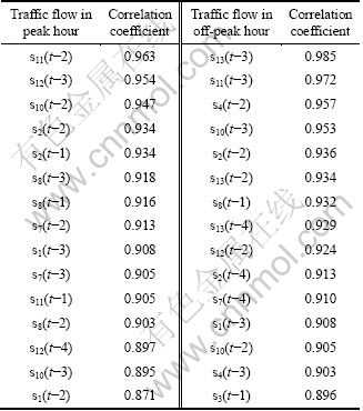
In addition, the Pearson correlation coefficients should be calculated. As mentioned in pre-selection procedure, the chosen detectors in Speak and Soff-peak with different time lags such as {(t), (t-1), ��, (t-d)} should be considered. In this work, d is set to be 5 for simplicity. Table 1 lists the top 15 most correlated traffic flows and their corresponding correlation coefficients with traffic flow at Detector 5 in peak and off-peak hour, respectively. It is easily noticed that the traffic flows with different time lags have a certain relationship with the target detector data.
Table 1 Fifteen most correlated traffic flows at Detector 5 in peak and off-peak hour
Subsequently, the forward stepwise regression was used to choose the most relevant data as the ��cause nodes�� set Sd. Then, after deriving the estimation formulation, the traffic data of the selected ��cause nodes�� were used to estimate the traffic condition at Detector 5.
To understand the performance of the pre-selection ��cause nodes�� space-time model, it is important to compare it with other estimators. In particular, three baseline traffic condition estimators were considered: The first one is the space time ARMA model without pre-selection procedure; The second one is the nearest neighbor regression model, which only considers the traffic condition of neighbors at current time with constrained area, and is trained with the maximum likelihood method; The third one is the stepwise linear regression model, which only takes into account the traffic condition at current time, but without the area constrained.
In this work, SPSS (Version 16.0.0) is selected to implement the models because of its good characteristics in statistics and simple to use. The ��Time Series�� and ��Regression�� statistical programs are used to perform the models.
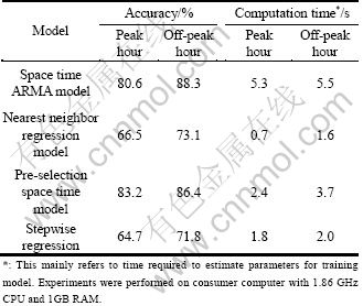
The accuracy and computation time of the four estimation methods are shown in Table 2. With the given experiment results, it can be noticed that the accuracy of the present model is higher than that of space time ARMA model in peak hour, but a little lower in off-peak hour. However, the space time ARMA model spends more computation time, which does not include the wasted time of model identification. The computation time of the nearest neighbor regression and stepwise regression model is much shorter than that of the present model, but the accuracy is rather lower. Furthermore, accuracy of 83.2% and 86.4% in the present model in peak and off-peak hour can be obtained, respectively, which represents the good accuracy and stability enough to achieve the actual demand.
Table 2 Experimental comparison results of four estimation models
6 Conclusions
1) A pre-selection space time model is proposed to estimate the traffic condition for the poor-data-detector and non-detector locations. The experimental results with the actual data demonstrate that the model is accurate and effective enough compared with other three models.
2) The model would also be suitable for the spatial distribution of the detectors. Since the traffic condition can be estimated accurately enough using the neighboring data, there is no need to install the detectors there, which can also reduce the construction costs.
3) Several factors should be researched and addressed for developing more robust estimation algorithms in the future. Firstly, the correlation of the traffic flow should be explored to get a more accurate coefficient. Secondly, applying the best historical data set as a seed to train the model should also be focused on.
References
[1] LIU Yi, SHA Man. Research on prediction of traffic flow at non-detector intersections based on ridge trace and fuzzy linear regression analysis [C]// Proceedings of International Conference on Computational Intelligence and Security. Washington D C: CPS, 2009: 571-575.
[2] WANG Yi-bing, PAPAGEORGIOU M, MESSMER A. Real-time freeway traffic state estimation based on extended kalman filter: A case study [J]. Transportation Science, 2007, 41(2): 167-181.
[3] SMITH B L, DEMERTSKY M J. Short-term traffic flow prediction: Neural network approach [J]. Transportation Research Record, 1994(1453): 98-104.
[4] SMITH B L, WILLIAMS B M, OSWALSD R K. Comparison of parametric and nonparametric models for traffic flow forecasting [J]. Transportation Research Part C: Emerging Technologies, 2002, 10(4): 303-321.
[5] WILLIAMS B M, HOEL L A, Modeling and forecasting vehicular traffic flow as a seasonal arima process: Theoretical basis and empirical results [J]. Journal of Transportation Engineering, 2003, 129(6): 642-672.
[6] HAN Chao, SONG Su. A review of some main models for traffic flow forecasting [C]// Proceedings of International IEEE Conference on Intelligent Transportation Systems. Shanghai: IEEE, 2003: 216-219.
[7] ZHANG He, WANG Wei, GU Huai-zhong. Application of cluster analysis and stepwise regression in predicting the traffic volume of lanes [J]. Journal of Southeast University (English Edition), 2005, 21(3): 359-362.
[8] KAMARIANAKIS Y. Spatial time series modeling: A review of the proposed methodologies [R]. The Regional Economics Applications Laboratory. 2003.
[9] KAMARIANAKIS Y, PRASTACOS P. Space-time modeling of traffic flow [J]. Computers and Geosciences, 2005, 31(2): 119-133.
[10] MIN W, WYNTER L, AMEMIYA Y. Real time road traffic prediction with spatio-temporal correlations [J]. Transportation Research Part C: Emerging Technologies, 2011, 19(4): 606-616.
[11] SUN Shi-liang, ZHANG Chang-shui. The selective random subspace predictor for traffic flow forecasting [J]. IEEE Transactions on Intelligent Transportation Systems, 2007, 8(2): 367-373.
[12] PFEIFER P E, DEUTSCH S J. Variance of the sample-time autocorrelation function of contemporaneously correlated variables [J]. SIAM Journal of Applied Mathematics: Series A, 1981, 40(1): 133-136.
[13] PFEIFER P E, DEUTSCH S J. A three-stage iterative procedure for space-time modeling [J]. Technometrics, 1980, 22(1): 35-47.
[14] GIACOMINI R, GRANGER C W J. Aggregation of space time processes [J]. Journal of Econometrics, 2004, 118(1): 7-26.
[15] JIA Li-min. Study on the novel and intelligent magnetic detectors [R]. Beijing: Beijing Jiaotong University and Beijing Traffic Management Bureau Report, 2008. (in Chinese)
[16] KINDZERSKE M D, NI D H. Composite nearest neighbor nonparametric regression to improve traffic prediction [J]. Transportation Research Record: Journal of the Transportation Research Board, 2007(1993): 30-35.
[17] GUYON I, ELISSEEFF A. An introduction to variable and feature selection [J]. Journal of Machine Learning Research, 2003(3): 1157-1182.
[18] SUN Xiao-liang. Research on traffic state forecasting towards urban freeway [D]. Beijing: Beijing Jiaotong University, 2009. (in Chinese)
(Edited by HE Yun-bin)
Foundation item: Project(D101106049710005) supported by the Beijing Science Foundation Program, China; Project(61104164) supported by the National Natural Science Foundation, China
Received date: 2011-02-25; Accepted date: 2011-05-19
Corresponding author: JIA Li-min, Professor; Tel: +86-10-51686441; E-mail: jialm@vip.sina.com
Abstract: A pre-selection space time model was proposed to estimate the traffic condition at poor-data-detector, especially non-detector locations. The space time model is better to integrate the spatial and temporal information comprehensibly. Firstly, the influencing factors of the ��cause nodes�� were studied, and then the pre-selection ��cause nodes�� procedure which utilizes the Pearson correlation coefficient to evaluate the relevancy of the traffic data was introduced. Finally, only the most relevant data were collected to compose the space time model. The experimental results with the actual data demonstrate that the model performs better than other three models.
