

Simulation analysis on three-dimensional slope failure under different conditions
ZHANG Ke1, CAO Ping1, LIU Zi-yao1, HU Hui-hua2, GONG Dao-ping2
1. School of Resources and Safety Engineering, Central South University, Changsha 410083, China;
2. Hunan Provincial Communication Planning Survey and Design Institute, Changsha 410008, China
Received 23 September 2010; accepted 5 January 2011
Abstract:
The failure mechanism of two-dimensional (2D) and three-dimensional (3D) slopes were investigated by using the strength reduction method. An extensive study of 3D effect was conducted with respect to boundary conditions, shear strength and concentrated surcharge load. The results obtained by 2D and 3D analyses were compared and the applicable scope of 2D and 3D method was analyzed. The results of the numerical simulation show that 3D effect is sensitive to the width of slip surface. As for slopes with specific geometry, 3D effect is influenced by dimensionless parameter c/(��Htanf). For those infinite slopes with local loading, external load has the major impact on failure mode. For those slopes with local loading and geometric constraints, the failure mode is influenced by both factors. With the increase of loading length, boundary condition exerts a more significant impact on the failure mode, and then 2D and 3D stability charts are developed, which provides a rapid and reliable way to calculate 2D and 3D factor of safety without iteration. Finally, a simple and practical calculation procedure based on the study of 3D effect and stability charts is proposed to recognize the right time to apply 2D or 3D method.
Key words:
three-dimensional slope; slope stability; three-dimensional effect; strength reduction method; failure mechanism;
1 Introduction
In slope stability analysis, two-dimensional (2D) method is usually employed under the assumption of plane strain condition, which is applied to the case that the slip surface is wide enough compared with the cross-sectional dimension. However, slope failure is often in three-dimensional (3D) form due to the complicated geological conditions as follows: 1) potential slip surface is constrained by physical boundaries, including excavation boundaries and heterogeneity in the soil properties; 2) the slope is imposed on load with limited area. Therefore, 3D analysis could offer a reflection on the actual state of slopes. A lot of research has demonstrated that the safety of 2D factor is conservative and smaller than 3D factor.
There are various progresses on 3D slope stability analysis. DUNCAN [1], GRIFFITHS and MARQUEZ [2] have respectively summarized the literature in different periods. 3D limit equilibrium methods including Swedish method [3], Bishop method [4], Janbu method [5], Spencer method [6-7] and Morgenstern-Price method [8] are extensions of 2D slice methods. Compared with 2D methods, most existing 3D limit equilibrium methods rely on more assumptions, which becomes the obstruction of 3D methods to be widespread in actual project. 3D variational calculus methods [9] and 3D limit analysis methods [10-12] possess stricter theoretical basis and thus they take a further step than 3D limit equilibrium methods. In addition, the above methods are all involved in search for critical slip surface. The optimized search algorithm for 2D critical slip surface is mature. But for 3D slope, the optimization problem encounters serious challenges with a substantial increasing number of variables.
Numerical simulation methods with deformation characteristics of soil considered, including finite element method and finite difference method, can actually reflect the stress and strain state of geotechnical engineering. In recent years, numerical simulation methods of 2D slope have been widely accepted [13-14]. However, numerical simulation methods of 3D slope have more advantages than 3D limit equilibrium methods that the former can analyze the state of 3D slope stability under complex geological and working conditions. CHUGH [15] carried out extensive research into 3D slope stability under different boundary conditions and indicated that an acceptable 3D solution depended on reasonably boundary conditions of numerical models. GRIFFITHS and MARQUEZ[2] researched the impacts of vertical boundary to sloping boundary and introduced variable strength parameters across the slope in the out-of-plane direction. WEI et al [16] conducted an extensive comparison between 3D limit equilibrium method and strength reduction method and the results obtained by these two methods were generally in good agreement. WEI et al [16] also pointed out that 3D strength reduction method was sensitive to the convergence criterion, boundary conditions and the design of mesh. Therefore, parameters of numerical models should be carefully chosen for 3D analysis.
However, the study on error analyses between 2D and 3D method is seldom deliberated. One of the main disadvantages of 3D strength reduction method is the long computing time required. When 2D analysis has little difference in error from 3D analysis, the former can replace the latter. In this work, through thousands of 3D examples, 3D effect of boundary conditions, shear strength parameters and external load were systematically analyzed. And then through the comparison between 2D and 3D methods, the failure mechanism of 3D slope was revealed. Furthermore, by means of error analyses, the calculation process of slope stability was proposed, which provided a simple and practical way to determine the applicable scope of 2D and 3D methods.
2 Three-dimensional effect of boundary conditions
A homogeneous slope serves as an example taken from Ref. [17], and its height H and angle �� are 5 m and 26�� (1:2), respectively, the 2D cross-section of which is shown in Fig. 1. The soil parameter values are listed as follows: unit weight ��=17.64 kN/m3, cohesion c=9.8 kPa, friction angle f=10��, elastic modulus E=100 MPa and Poisson ratio ��=0.3. Factor of safety is solved by means of built-in command solve fos of FLAC3D. Maximum shear strain increment is chosen to define critical failure surface. The left and right boundaries of 2D numerical model are constrained by vertical rollers, and bottom boundary is constrained by both horizontal and vertical directions. The model, in which Morh-Coulomb failure criterion and non-associated flow rule are used, is built large enough to reduce the size effect, with the length from slope toe to the left boundary 1.5H, the length from slope crest to the right boundary 2.5H, and the length from slope crest to the bottom boundary 2H, as shown in Fig. 2.
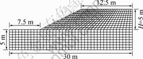
Fig. 1 Dimensions of 2D cross-section slope
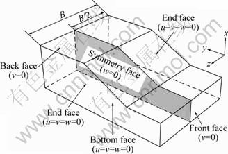
Fig. 2 Schematic diagram of boundary conditions of 3D model
u, v and w respectively represent the displacement in x, y and z directions. For 3D numerical model, the bottom surface of the slope is fully constrained (u=v=w=0), and the back and front face are constrained by the displacement in the y direction (v=0) as seen in Fig. 2. Boundary conditions of end faces play an important role in 3D stability analysis. If end faces of the slope are constrained by the displacement in the z direction (w=0), shear resistance will disappear in both faces, and the case mentioned above will turn 3D calculation into plane strain solution, thus, its result equals that of 2D, which could not offer a reflection on 3D effect, as shown in Fig. 3(a). In order to provide shear resistance for 3D slip surface, the end faces of the slope are all fully constrained in three directions (u=v=w=0), as shown in Fig. 3(b). Symmetry is assumed for simplicity so that only half of the slope needs to be analyzed. As shown in Fig. 3(c), symmetry plane is constrained by displacement in the z direction. Figures 3(b) and (c) show that the shapes of the failure surfaces are different at different cross sections in the z direction.
2D analysis is popular in engineering calculation and it is applied to the slope with infinite width. However, the width of failure mass is finite in engineering practice owing to the complex geometry or boundary conditions. In this section, the impact of widths of slip surface on 3D effect is investigated and the comparison between 2D and 3D analyses is shown in Figs. 4 and 5 to determine the applicable scope of 2D analysis. Relative difference, ��, which is used to quantitatively reflect 3D effect, represents relative difference between the factors and safety obtained by 2D and 3D methods, and it is expressed as:
![]() (1)
(1)
where F3D and F2D represent 3D and 2D factors of safety, respectively.
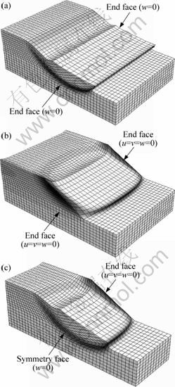
Fig. 3 End faces constrained by displacement in z direction (a), three directions (b) and three directions with assumed symmetry (c) in deformed meshes of 3D slopes
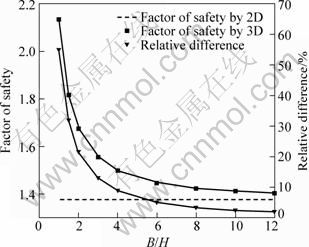
Fig. 4 Factors of safety and relative differences with different widths of slip surfaces
With the increase in width of slip surface B, F3D decreases while 3D effect gets less remarkable. F3D tends to be the plane strain solution with B/H��10. Additionally, from Fig. 5, it is interesting to find that slip surfaces on symmetry plane remain little changed with different widths of slip surface. So, the depth of landslide obtained by 2D method can be estimated.
3 Three-dimensional effect of strength parameters
Mohr-Coulomb criterion is mainly adopted for the numerical analysis of geotechnical engineering, which considers cohesion and friction angle as the main strength parameters of soil. In this section, the influence of soil strength parameters on 3D effect of slopes is investigated by changing the value of cohesion and friction angle. The slope from Ref. [17] is still selected as the analysis example, the widths of which are 10, 20 and 30 m, consequently (i.e., B/H=2, 4 and 6).
The variable cohesion varies from 0 to 20 kPa (i.e., c=0, 2, 4, 6, ��, 16, 18, 20 kPa) while other parameters remain constant. The results under the above conditions obtained by 2D and 3D analyses are shown in Figs. 6 and 7. F2D and F3D increase with the increase of cohesion, and the relative difference between two methods also increases, namely, 3D effect is more remarkable. Then the failure mode of slope changes from shallow slip to deep slip.
The variable friction angle varies from 0 to 20�� (i.e., f=0, 2��, 4��, 6��, ��, 16��, 18��, 20��) while other parameters remain constant. The results under the above conditions obtained by 2D and 3D analyses are shown in Figs. 8 and 9. F2D and F3D increase with the increase of friction angle, but the relative difference between the two methods decreases (namely, 3D effect is more weaken) during this process. And the failure mode of slope changes from deep slip to shallow slip.
Through the parametric study of shear strength, it is noticed that 3D effect (i.e., relative difference between 2D and 3D methods) is mostly influenced by locations of slip surfaces. When shallow failure happens, the value of relative difference is low and 3D effect is not remarkable. In this study, d denotes the depth of slip surface. 3D effect is more pronounced as the ratio of the depth to width of failure mass d/B increases. For soil with c=0 and d/B=0, good agreement between F2D and F3D is reached. When d/B<0.07, the relative difference �� is less than 5%, but �� exceeds 50% once d/B��0.45. So, d/B can be the qualification for reasonable selection of 2D or 3D method.
In order to determine whether 3D analysis is necessary or not, the steps are taken as follows:
1) The factor of safety and the corresponding critical slip surface with 2D method are calculated and the depth of failure mass d is determined.
2) The width of potential slip surface through field survey is estimated.
3) If d/B��0.07, it is shown that relative difference between 2D and 3D method is within the acceptable range and the result obtained by step 1 can be executed directly. If d/B exceeds 0.07, 3D effect should not be ignored and the calculation with 3D analysis is necessary.

Fig. 5 Slip surfaces with different widths of slip surfaces: (a) 2D; (b) 3D, B/H=2; (c) 3D, B/H=4; (d) B/H=8; (e) 3D, B/H=10
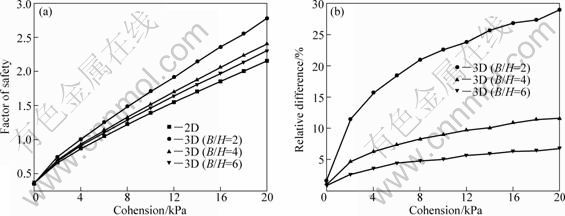
Fig. 6 Factors of safety (a) and relative differences (b) with different cohesions

Fig. 7 Slip surfaces with different cohesions when B/H=4: (a) 0; (b) 4 kPa; (c) 8 kPa; (d) 12 kPa; (e) 16 kPa; (f) 20 kPa

Fig. 8 Factors of safety (a) and relative differences (b) with different friction angles
4 Stability charts for three-dimensional slope
4.1 Development of stability charts
Slope stability charts provide a rapid and reliable way to calculate factors of safety, which can be used for preliminary analysis and back-calculation. Based on the conclusions of relationship among slope parameters (H, ��, c, f and ��), many researchers have developed stability charts of 2D slope, which require a iterative procedure [18]. The method introduced by BELL [19] without any iteration required seems to be the most convenient method. It is proposed that F/tanf is given as a function of c/(��Htan f). MICHALOWSKI [20] used BELL��s method to develop charts for 2D slopes that took pore water pressure and seismic load into consideration. Recently, MICHALOWSKI [12] has extended 2D limit analysis method to 3D method, and the stability charts for 3D slope failures are presented by this useful method. There are other stability charts of 3D slope presented by other researchers, such as LESHCHINSKY and BAKER [9], GENS et al [3] and CENG [10]. The charts above are all based on 3D limit equilibrium method or limit analysis method on the assumptions of internal forces distribution and the shape of slip surface. However, strength reduction method does not rely on the assumptions mentioned above and the critical slip surface and the corresponding factor of safety can be automatically obtained. Therefore, it is more scientific and efficient to construct the stability charts of 3D slope with BELL��s concept and strength reduction method. The dimensionless parameter �� is defined as:
![]() (2)
(2)
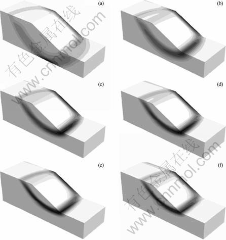
Fig. 9 Slip surfaces with different friction angles when B/H=4: (a) 0; (b) 4��; (c) 8��; (d) 12��; (e) 16��; (f) 20��
On the purpose of representing 3D effect, B/H is also added to the stability charts of 3D slope, the values are 1.0, 1.5, 2, 3, 4 and 6 each times. And the values of 15��, 30��, 45��, 60�� and 75�� are assigned to slope angle. Under inhomogeneous condition, it is necessary to approximate the real condition with an equivalent homogenous slope.
As the same value of tanf used in 2D and 3D analyses, relative difference can also be redefined as:
![]() (3)
(3)
From Eq. (3) and Fig. 10, c/(��Htan f) is the control factor for 3D effect, which can quantitatively reflect the relative difference between F2D and F3D. And the treatment above is more convenient and effective than evaluating the value of d/B.
4.2 Numerical results
The design charts of calculating 2D and 3D factors of safety and relative differences are shown in Fig. 10. It is indicated that F3D decreases with the increase of B/H. When the value of B/H is 1, the corresponding relative difference may exceed 50% but when the value is 6, the corresponding relative difference is less than 10%. As �� increases, the factor of safety and relative difference both increase. When the value of �� is between 0 and 0.1, the relationship between �� and F/tanf is nonlinear and linear relationship is more obvious as �� increases.

Fig. 10 Stability charts for 3D slope with different slope angles: (a), (a') 15��; (b), (b') 30��; (c), (c') 45��; (d), (d') 60��; (e), (e') 75��
From Figs. 10 and 11, it is indicated that F3D decreases as the slope angle increases. If slope angle is not equal to the specific value (i.e., 15��, 30��, 45��, 60�� and 75��), the factor of safety can be computed by linear interpolation method. When ��<60��, relative difference shows a downward tendency with the increase of �� and relative difference slightly increases with the continuous increase of ��. The higher the value of �� is, the more pronounced the downward tendency is.

Fig. 11 Relationship between F/tanf (a) and relative difference (b) with slope angle (B/H=4)
For cohesionless soil, CHEN and CHAMEAU [6] concluded that the case with F3D/F2D<1 might happen, which was disagreed by HUTCHINSON and SARMA [21], CAVOUNIDIS [22] and HUNGR [4]. They indicated that F3D was always greater than or equal to F2D. CHEN and CHARMEAU��s error was pointed out by CAVOUNIDIS [22]. The result obtained by 3D strength reduction method was somewhat different from what the predecessors concluded. Figure 12 shows that F3D is slightly less than F2D in certain circumstances, especially with higher values of slope angle �� and B/H. F3D is always greater than F2D when ��=15��, but always lower than F2D when ��=75��. With the increase of B/H, relative difference between F3D and F2D decreases, apart from the condition that �¡�75��.
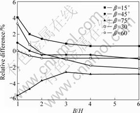
Fig. 12 Relative differences with cohesionless soils
4.3 Example
4.3.1 MICHALOWSKI slope
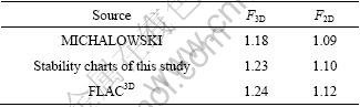
Example 1 is a homogeneous slope taken from Ref. [12], with height of 15 m and slope ratio of 1:1. The soil parameters are: ��=18 kN/m3, c=20 kPa, f=20��, and the width is restricted to 30 m (B/H=2). To use the new charts for 3D slope, first it is calculated, ![]() . It is found that F3D/tanf=3.38 and
. It is found that F3D/tanf=3.38 and ![]() from Fig. 10(c). And then F3D=3.38tan20��=1.23 and F2D=3.03tan20��=1.10. The results obtained by MICHALOWSKI analysis are listed in Table 1. The factors of safety are also evaluated by FLAC3D to justify the applicability of stability charts. The results coincide well with the ones calculated by MICHALOWSKI and FLAC3D analysis.
from Fig. 10(c). And then F3D=3.38tan20��=1.23 and F2D=3.03tan20��=1.10. The results obtained by MICHALOWSKI analysis are listed in Table 1. The factors of safety are also evaluated by FLAC3D to justify the applicability of stability charts. The results coincide well with the ones calculated by MICHALOWSKI and FLAC3D analysis.
Table 1 Comparison of results from different methods for example 1
4.3.2 ZHANG slope
Example 2 is a homogeneous slope taken from Ref. [7], with the height of 12 m and slope angle of 1:2 (26.6��). The soil parameter values are ��=18.8 kN/m3, c=29 kPa and f=20��. Through the calculation, B/H=6 and ��=0.35 are obtained. From Figs. 10(a) and (b), for slopes with angles of 15�� and 30��, F3D/tanf=8.58 and F3D/tanf=5.51, respectively, and their corresponding factors of safety F3D=8.58tan20��=3.12 and F3D= 5.51tan20��=2.00, respectively.
With linear interpolation method, 3D factor of safety with slope angle of 26.6��can be computed as:
![]() . For this
. For this
example, F3D computed by 3D limit equilibrium [7] and 3D limit analysis method [11] are 2.122 and 2.262 each time, respectively.
4.3.3 Open pit slope of Jiagou aluminum mine
Example 3 is an eastern slope of Jiagou open-pit aluminum mine, with slope angle of 41.3�� and height of 32 m. After sampling in mining area and testing physical and mechanical parameters, equivalent soil parameters are ��=18.50 kN/m3, c=40 kPa and f=27��. As the same calculation process above, it is obtained that ��=0.13, and then the corresponding values of F/tanf for 30�� and 45�� slope are read from Fig. 10. The factors of safety for 41.3�� slope by using linear interpolation method are computed, as shown in Fig. 13. The relationship between F3D and B/H can be obtained, which provides practical guidance for slope stability analysis. 3D factor of safety can be easily determined once the potential width of slip surface is estimated.
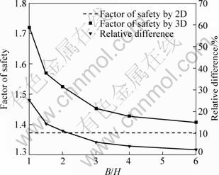
Fig. 13 Factors of safety for example 3
5 Three-dimensional effect of concentrated surcharge load
2D analysis is just applicable to slope with infinite width (or infinite slope) imposed on loading with infinite length. However, loading length is finite in engineering practice. If the infinite slope is imposed on external load, 3D failure will appear even though the potential slip surface is not constrained by physical boundaries. Suppose the slope is imposed with rectangular loading that is uniformly distributed, as shown in Fig. 14. The loading q is just at the edge of slope vertex, with loading intensity of 50 kPa and loading width of 2 m (represented by D). And if the failure is induced by external load, the width of slip surface B may be lower than the width of model, W.

Fig. 14 Slope with surcharge loading
For slope with infinite width, the width is far greater than its cross-sectional size, with constraint of displacement in normal direction at end faces (w=0). Loading length L is 2, 4, 6, 8, 10, 12, 16, 20, 30 and 40 m each time. When the value of L is lower than 20 m, the model width is chosen as 40 m. When value of L is higher than 20 m, the model width is chosen as 2L. The results calculated by 2D and 3D analyses with different loading lengths are shown in Figs. 15 and 16. F3D declines with the increase of loading length and 3D effect gradually weakens and it tends to be the plane strain solution when L/H��6. The failure mode of infinite slope under the action of loading is mainly controlled by external load.
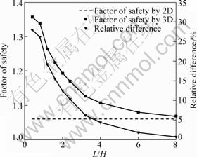
Fig. 15 Factors of safety with different loading lengths for infinite slope
For slope with concentrated surcharge load, the width of potential landslide may be restricted by boundary conditions, in which case it is different from that of the infinite slope. Suppose the slope model with width of 20 m, end faces are fully constrained in three directions (u=v=w=0) and L varies from 2 to 20 m (i.e., L=2, 4, 6, 8, 10, 12, 14, 16, 18 and 20 m). The results are compared with those of infinite slope, as seen in Figs. 16 and 17. When L��4 m, 3D slip surface of infinite slope cannot be formed. As to the slope with finite width (or finite slope, W=20 m and u=v=w=0 at the end faces of the model), 3D failure can always be found, and the width of slip surface is equal to the model width for L��4 m. Consequently, 3D factors of safety are different from each other. When L��4 m, the factor of safety varies slightly, and the relative difference is less than 0.3%. For those slopes with local loading and geometric constraints, the failure mode is influenced by loading and constraint.
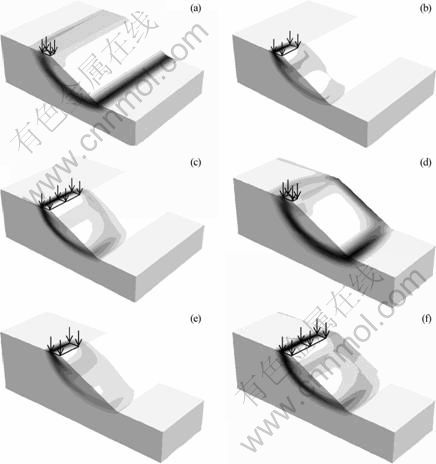
Fig. 16 Slip surfaces with different loading lengths: (a) Infinite slope, L=2 m; (b) Infinite slope, L=8 m; (c) Infinite slope, L=16 m; (d) Finite slope, L=2 m; (e) Finite slope, L=8 m; (f) Finite slope, L=16 m
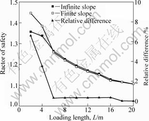
Fig. 17 Factor of safety with infinite slope and finite slope (W=20 m and u=v=w=0 at model ends)
The influence of widths of model W upon boundary effect are studied with w=0 and u=v=w=0 at the end faces of the model, the results are listed in Tables 2 and 3.
Table 2 Factors of safety and failure modes with different model widths when L=8 m
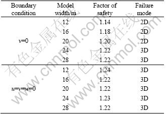
Table 3 Factors of safety and failure modes with different model widths when L=16 m
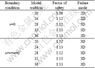
1) If the end faces are constrained by the displacement in normal direction. In the case of L=8 m, when the value of W increases in the 12-24 m range, F3D with w=0 at the end faces increases and remains constant with further increase of W. 3D failure of this boundary condition does not appear until W��24 m. In the case of L=16 m, when the value of W increases in the 20-24 m range, F3D with w=0 at end faces increases, and remains constant with further increase of B. And 3D failure would not happen until W��28 m. Therefore, the width of the model mentioned above is large enough in size to result in 3D failure for infinite slope. So, the width of infinite slope can meet the demands of calculation in this section.
2) If the end faces are constrained by the displacement in three directions, in spite of the variance in widths of the models, 3D factors of safety and slip surfaces approximately remain the same.
In the view of the above analysis, 3D failure is greatly influenced by the model width under the boundary condition when w=0. So, a large size is required for infinite slope (i.e. influence of physical boundaries omitted), and the case is also mentioned by WEI et al [16]. Hence, the boundary condition that u=v=w=0 at end faces is recommended, which can reduce the model size effectively. It is worth noting that the treatment is just appropriate for infinite slope with surcharge loading under the conditions that 3D failure results from external load and the model width is greater than that of failure mass in size.
6 Calculation procedure for slope stability analysis
In terms of the study on failure mechanism of 3D slope and the comparison with 2D analysis results mentioned above, convenient and pragmatic calculation procedure on slope stability analysis is proposed, as shown in Fig. 18.
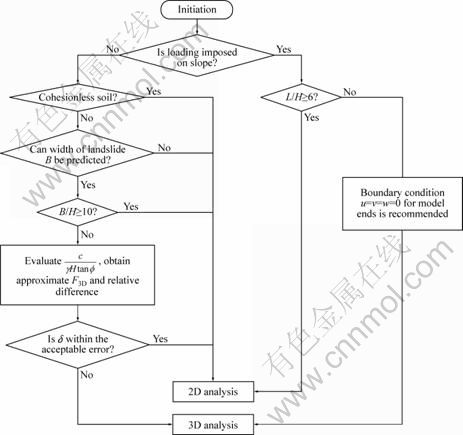
Fig. 18 Calculation procedure for slope stability analysis
As for the slope without loading, 2D analysis method can be employed because there is little error between 2D and 3D analysis under the following conditions:
1) For slope of cohesionless soil, F3D=F2D, both of which are approximately equal to the theoretical solution tan f/tan ��;
2) The width of potential failure mass B cannot be estimated and the slope is of high level of security;
3) B/H��10;
4) Through evaluating dimensionless parameter
![]() , approximate F3D and relative difference �� can
, approximate F3D and relative difference �� can
be obtained from Fig. 10. If �� is within the acceptable error (5% in general), then 2D analysis method can be adopted.
If loading is imposed on slope, 2D method can be employed as long as L/H��6.
In other cases, 3D method should be adopted. For infinite slope with local loading, it is suggested that the displacement at end faces should be constrained in three directions in order to reduce the model size.
7 Conclusions
1) Failure mechanism of 3D slope is greatly affected by the boundary conditions. If the width of the potential failure is physically limited, the displacement should be constrained in three directions at end faces. The failure under the condition that B/H��10 can be considered close to the plane strain solution.
2) As for slopes with specific geometry (specified values of B and ��), dimensionless parameter ![]() controls 3D effect. The higher the value of
controls 3D effect. The higher the value of ![]() is, the more the pronounced 3D effect is. F3D effect is generally higher than F2D. But in certain circumstances, F3D effect for cohesionless soil may be slightly lower than that of F2D, especially with higher values of �� and B/H.
is, the more the pronounced 3D effect is. F3D effect is generally higher than F2D. But in certain circumstances, F3D effect for cohesionless soil may be slightly lower than that of F2D, especially with higher values of �� and B/H.
3) 3D failure of infinite slope is easily formed with load placed on the slope crest. The failure under the condition that L/H��6 can be considered close to the plane strain solution. For the slope that is also affected by geometric constraints, it is interesting to find that the result agrees well with that of infinite slope, but the slope with physical constraints has a smaller size.
4) F3D and F2D are functions of dimensionless parameter![]() and B/H, their relative difference can be plotted in the form of stability charts and they can be easily and conveniently computed without iterative procedure. As for complicated slope, it is better to simulate the distribution of soil layer and the working conditions to reanalyze the slope stability by 3D strength reduction method.
and B/H, their relative difference can be plotted in the form of stability charts and they can be easily and conveniently computed without iterative procedure. As for complicated slope, it is better to simulate the distribution of soil layer and the working conditions to reanalyze the slope stability by 3D strength reduction method.
5) Based on the present study on failure mechanism of 3D slope and comparison between 2D and 3D analysis, the calculation procedure is presented. Under the condition that relative difference between F2D and F3D is within the acceptable range in engineering, and 2D method can be used. In other cases, it is suggested that 3D method should be used.
References
[1] DUNCAN J M. State of the art: Limit equilibrium and finite element analysis of slopes [J]. Journal of Geotechnical Engineering, ASCE, 1996, 122(7): 577-596.
[2] GRIFFITHS D V, MARQUEZ R M. Three-dimensional slope stability analysis by elasto-plastic finite elements [J]. Geotechnique, 2007, 57(6): 537-546.
[3] GENS A, HUTCHINSON J N, CAVOUNIDIS S. Three dimensional analysis of slides in cohesive soils [J]. Geotechnique, 1988, 38(1): 1-23.
[4] HUNGR O. An extension of Bishop��s simplified method of slope stability analysis to three dimension [J]. Geotechnique, 1987, 37(1): 113-117.
[5] HUNGR O, SALGADO F M, BYRNE P M. Evaluation of a three-dimensional method of slope stability analysis [J]. Canadian Geotechnical Journal, 1989, 26(4): 679-686.
[6] CHEN R H, CHAMEAU J L. Three-dimensional limit equilibrium analysis of slopes [J]. Geotechnique, 1983, 32(1): 31-39.
[7] ZHANG X. Three-dimensional stability analysis of concave slopes in plan view [J]. Journal of Geotechnical Engineering, ASCE, 1987, 114(6): 658-671.
[8] LAM L, FREDLUND D G. A general limit equilibrium model for three-dimensional slope stability analysis [J]. Canadian Geotechnical Journal, 1993, 30(6): 905-919.
[9] LESHCHINSKY D, BAKER R. Three-dimensional slope stability: End effects [J]. Soils and Foundations, 1986, 26(4): 98-110.
[10] CENG C Z. Three-dimensional slope stability analysis and support strategies for conical excavations [D]. Raleigh: Graduate Faculty of North Carolina State University, 1997.
[11] CHEN Z, WANG X, HABERFIELD C, YIN J H, WANG Y. A three-dimensional slope stability analysis method using the upper bound theorem, Part 1: Theory and methods [J]. International Journal of Rock Mechanics and Mining Sciences, 2001, 38(3): 369-378.
[12] MICHALOWSKI R L. Limit analysis and stability charts for 3D slope failures [J]. Journal of Geotechnical and Geoenvironmental Engineering, ASCE, 2010, 136(4): 583-593.
[13] GRIFFITHS D V, LANE P A. Slope stability analysis by finite element [J]. Geotechnique, 1999, 49(3): 387-403.
[14] CHENG Y M, LANSIVAARA T, WEI W B. Two-dimensional slope stability analysis by limit equilibrium and strength reduction methods [J]. Computers and Geotechnics, 2007, 34(3): 137-150.
[15] CHUGH A K. On the boundary conditions in slope stability analysis [J]. International Journal for Numerical and Analytical Methods in Geomechanics, 2003, 27(11): 905-926.
[16] WEI W B, CHENG Y M, LI L. Three-dimensional slope failure analysis by the strength reduction and limit equilibrium methods [J]. Computers and Geotechnics, 2009, 36(1-2): 70-80.
[17] GRECO V R. Efficient Monte Carlo technique for locating critical slip surface [J]. Journal of Geotechnial Engineering, ASCE, 1996, 122(7): 517-525.
[18] DUNCAN J M, WRIGHT S G. Soil strength and slope stability [M]. Hoboken, US: John Wiley & Sons, 2005: 265-280.
[19] BELL J M. Dimensionless parameters for homogenous earth slopes [J]. Journal of Soil Mechanics and Foundation Engineering Division, ASCE, 1966, 92(5): 51-65.
[20] MICHALOWSKI R L. Stability charts for uniform slopes [J]. Journal of Geotechnical and Geoenvironmental Engineering, ASCE, 2002, 128(4): 351-355.
[21] HUTCHINSON J N, SARMA S K. Discussion on three- dimensional limit equilibrium analysis of slopes [J]. Geotechnique, 1985, 35(2): 215.
[22] CAVOUNIDIS S. On the ratio of factors of safety in slope stability analyses [J]. Geotechnique, 1987, 37(2): 207-210.
��ͬ��������ά����ʧ�ȹ��ɵ���ֵģ��
�� ��1���� ƽ1��������1�����ݻ�2������ƽ2
1. ���ϴ�ѧ ��Դ�밲ȫ����ѧԺ����ɳ 410083��
2. ����ʡ��ͨ�滮�������Ժ����ɳ 410008
ժ Ҫ������ǿ���ۼ����о���ά����ά���µ�ʧ�Ȼ�����ͨ�������������������߽�������ǿ�Ȳ������¶����ص���άЧӦ�������ά���㷽���Ľ�����жԱȣ�ȷ����ά����ά���㷽�������÷�Χ����ֵģ��ļ�������������άЧӦ�Ի�����Ⱥ����У��������ض��ı��¼��γߴ磬��άЧӦ���������ٲ���c/(��Htan f)��Ӱ�졣�����¶����ܺ��ص��������£�����ʧ��ģʽ��Ҫ�ܵ����ص�Ӱ�졣������ͬʱ�ܵ������߽���¶��������õı��£�ʧ��ģʽ���ܵ����ߵ�Ӱ�죻���ź��س��ȵ����ӣ��߽�������Ӱ��������������������ά����ά�ı����ȶ�����ͼ�����Կ��١��ɿ���ȷ����ά����ά��ȫϵ�����Ҳ���Ҫ�κε���������ڱ�����άЧӦ�ͱ����ȶ�����ͼ���о����ܽ�һ��ʵ�õı��¼������̣��жϺ�ʱ�ò��ö�ά����ά���㷽����
�ؼ��ʣ���ά���£������ȶ�����άЧӦ��ǿ���ۼ������ƻ�����
(Edited by FANG Jing-hua)
Foundation item: Project (10972238) supported by the National Natural Science Foundation of China; Project (2010ssxt237) supported by the Excellent Doctoral Thesis Program of Central South University, China
Corresponding author: CAO Ping; Tel: +86-731-88879263; E-mail: pcao_csu@163.com
DOI: 10.1016/S1003-6326(11)61041-8
Abstract: The failure mechanism of two-dimensional (2D) and three-dimensional (3D) slopes were investigated by using the strength reduction method. An extensive study of 3D effect was conducted with respect to boundary conditions, shear strength and concentrated surcharge load. The results obtained by 2D and 3D analyses were compared and the applicable scope of 2D and 3D method was analyzed. The results of the numerical simulation show that 3D effect is sensitive to the width of slip surface. As for slopes with specific geometry, 3D effect is influenced by dimensionless parameter c/(��Htanf). For those infinite slopes with local loading, external load has the major impact on failure mode. For those slopes with local loading and geometric constraints, the failure mode is influenced by both factors. With the increase of loading length, boundary condition exerts a more significant impact on the failure mode, and then 2D and 3D stability charts are developed, which provides a rapid and reliable way to calculate 2D and 3D factor of safety without iteration. Finally, a simple and practical calculation procedure based on the study of 3D effect and stability charts is proposed to recognize the right time to apply 2D or 3D method.
