
J. Cent. South Univ. (2012) 19: 1600-1609
DOI: 10.1007/s11771-012-1182-3![]()
Identification of contamination source in water distribution network based on consumer complaints
TAO Tao(����)1, HUANG Hai-dong(�ƺ���)1, XIN Kun-lun(������)1, LIU Shu-ming(������)2
1. College of Environmental Science and Engineering, Tongji University, Shanghai 200092, China;
2. School of Environment, Tsinghua University, Beijing 100084, China
? Central South University Press and Springer-Verlag Berlin Heidelberg 2012
Abstract:
A new methodology was proposed for contamination source identification using information provided by consumer complaints from a probabilistic view. Due to the high uncertainties of information derived from users, the objective of the proposed methodology doesn��t aim to capture a unique solution, but to minimize the number of possible contamination sources. In the proposed methodology, all the possible pollution nodes are identified through the CSA methodology firstly. And then based on the principle of total probability formula, the probability of each possible contamination node is obtained through a series of calculation. According to magnitude of the probability, the number of possible pollution nodes is minimized. The effectiveness and feasibility of the methodology is demonstrated through an application to a real case of ZJ City. Four scenarios were designed to investigate the influence of different uncertainties on the results in this case. The results show that pollutant concentration, injection duration, the number of consumer complaints nodes used for calculation and the prior probability with which consumers would complaint have no particular effect on the identification of contamination source. Three nodes were selected as the most possible pollution sources in water pipe network of ZJ City which includes more than 3 000 nodes. The results show the potential of the proposed method to identify contamination source through consumer complaints.
Key words:
water distribution network; contamination source; identification; consumer complaints��
1 Introduction
Since injections of a pollutant into a water distribution network may have a dramatic effect on public health and on other aspects such as economical aspect, more and more attentions have been given to the problem of identifying the location and release history of contamination source. There may be many routines in which pollutant can enter a water distribution system. In general, they can be grouped into accidental routines (e.g., back flow of contaminated water from consumer facilities) and intentional routines (e.g., terrorist attack). Likewise, the problem of identification can be solved directly or indirectly [1].
As the problem of identification is of great importance, especially for user��s health, various researchers have developed many methodologies for contamination source identification. These methodologies can be summed up into two sorts roughly [2]: a water back-tracking methodology, which regards source identification as an inverse problem of the standard water quality simulation, and a water quality forward simulation methodology, which primarily makes use of predictor-corrector algorithm to identify the sources location and their release histories. As to the water back-tracking methodology, since SHANG et al [3] presented particle backing algorithm based on an input- output model, many methodologies based on this model have been proposed to solve the source identification problem [4-5]. And with respect to the water quality forward simulation, various methodologies based on different procedures have been reported in recent years [6-8]. However, these aforementioned researchers mainly focused on using sensor data to identify contamination source, and few attentions have been given to using information provided by consumer complaints to locate the pollution source. There is no doubt that source identification through sensor data can allow an effective response to reduce and avoid the potential adverse impacts in time. Nevertheless, if it cannot identify the contamination source due to lack of monitoring station, using other available data to identify the source would become more important to identify and respond to the contamination event as soon as possible, even though it would be possible to result in non-unique solutions. In this work, a new methodology is proposed to solve the contamination source identification problem from a probabilistic view. The most significant characteristic of the methodology proposed herein is that the data of monitoring station are not needed, and information derived from consumer complaints is used for identifying the contamination source for the first time. However, the objective of source identification here doesn��t aim to capture an exact or unique solution, but to demonstrate a few most possible pollutant sources differed from many ��candidate�� nodes through some particular procedures. The methodology is designed to be a simple and easy-use tool for water utilities for a fast identification of the contamination source, based on hypotheses and with a high computational efficiency.
2 Methodology
Just as Bayesian belief networks (BBN) [9-10], based on Bayesian theorem, the proposed methodology also solves the problem from a probabilistic view.
Bayesian theorem can typically be stated as
 (1)
(1)
where P(Bi|A) is the posterior probability of Bi given that event A is true; P(A|Bi) is the probability of event A given that Bi is true; P(Bi) is the prior probability of Bi which may make event A become true; P(Bj) is the prior probability of Bj which may make event A become true; P(A|Bj) is the probability of event A given that Bj is true; n is the number of factor which may influence event A.
Based on probability reasoning, in general, BBN can be presented as a directed acyclic graph model, in which a node represents a random variable and an arc represents assertions of conditional independence. As shown in Fig. 1, in the alarm BBN model, in the case of given E, variable A can be considered to be conditionally independent of variables B, C and D.

Fig. 1 Alarm network model
In reality, Bayesian theorem can be interpreted as such a procedure, whose aim is to calculate the probability of one factor that may cause the event and thereby to demonstrate the reliability of the factor, given that the event has been true. In the field of drinking water supply, several researchers have utilized Bayesian approaches for a number of applications [11-12]. In contrary to Bayesian theorem, the theorem, on which the proposed methodology is based, aims to calculate the possibility of the event occurring, given that a number of factors may result in the occurrence of event. And the theorem can be stated as
![]() (2)
(2)
where P(A) is the total probability, given that A is true.
Equation (2) is typically termed total probability formula, in which factors influencing event A are mutually exclusive. A directed acyclic graph just like a BBN to represent this theorem is constructed and shown in Fig. 2.

Fig. 2 Schematic diagram based on total probability formula
Actually, there are no differences between Fig. 2 and Fig. 1 to some extent, and the nodes and arcs of them represent the same significance. A major difference is that the purpose that the diagram seeks to reflect. Figure 1, a simple Bayesian belief network structure, represents the causal relationships among the nodes; while Fig. 2 demonstrates the number of factors that can lead to event occurring and the relationships among these nodes. In this work, some nodes which might be the most possible intrusion sources are identified by the magnitude of probability of all ��candidate�� nodes. Prior probabilities are determined by using some common sense and expert knowledge, and posterior probabilities are derived from a series of calculations.
In this work, it is assumed that a conservative contamination goes into the network through a single point. The injection for each potential pollution node follows the following characteristics: the same pollutant intrusion concentration and the same injection duration. This methodology also assumes a complete mixing in each node and neglects the pollutant dispersion. The steps of the proposed method are as follows:
1) Determine a number of nodes where it is possible that the contamination intrusion occurs. In this work, EPANET 2.0 [13] is used to simulate hydraulics of the water distribution system. To acquire the hydraulic state of system at each hour, the knowledge of the network scheme and water demands are required at each time when the simulation is implemented. SANCTIS et al [14] developed a method called CSA methodology which only requires a binary sensor status over time to identify all possible locations. The details of CSA methodology is not presented here anymore. In fact, consumer complaints node play the same role as the sensors and the only difference between them is the accuracy of time when water quality becomes abnormal. However, because the CSA methodology requires real-time data while consumer complaints cannot provide available real-time data, some issues should be solved properly. Firstly, the possible contamination time can be estimated through supposing that consumers complain to water utilities within several hours after they find the water becomes abnormal. In this work, it is assumed that consumers would complain to water utilities within 2 h (Hypothesis 1), and the effect of different time when consumers would complain to water utilities would be discussed in the next section. Secondly, because the concentration of pollutant is also not available too, in order to identify all the possible contamination nodes, all the flow paths are treated equally setting threshold �� as small as possible (�š�0).
2) Determine the possible combinations of contamination time in which contamination event would occur at all the complaint nodes simultaneously. As stated above, it is impossible to obtain the exact contamination time from consumers. In a word, the contamination time is of uncertainty. To reduce and quantify such uncertainty, the possible contamination time of each complaint node is divided into several parts equally, and the possible combinations of contamination time when contamination event would occur at all the complaint nodes simultaneously are determined. In this work, 1 h is regarded as a unit which is used for dividing the possible pollution time of all the complaint nodes. The reasons why choose 1 h as the parameter are as follows: (1) if the time for dividing is too small, it would lose statistical significance; (2) if the time is too long, it cannot decline the uncertainty effectively. According to Hypothesis 1, the possible contamination time is divided into two parts, and the total number of combinations would be 2k (k is the number of consumer complaint nodes). To accord with the following steps, time obtained from users is required to further process. For example, a consumer complains to water utilities at 9:45. In terms of above assumption, the time of contamination occurring would be between 7:45 and 9:45, but in this work it is regarded that the event occurs between 8:00 and 9:45, for 45 min exceeds 30 min. In contrary, while the time is not 9:45 but 9:20, the event is considered to occur between 7:00 and 9:00, for 20 min is less than 30 min. The reasons why processing data like these are as follows: Firstly, it is necessary to be consistent with the following steps; Secondly, the impact of such process on the results can be reduced to some extent, because the probabilities are obtained by continuous multiplication. In order to better demonstrate the process, an example is illustrated below. Given that there are two nodes where consumers complain at 9:20 and 9:45 respectively, the possible pollution time would be 7:20-9:20 and 7:45-9:45 respectively according to the hypothesis proposed above. However, the possible combinations of consumer complaint time after further process are listed in Table 1.
Table 1 Possible combinations of consumer complaints time

3) Determine the probability of each combination of time P(A|Bj) (j=1 to n, n represents the total number of the time combinations of consumer complaints) of each potential intrusion location by computer simulation. In this work, it is assumed that a conservative contamination goes into the network through a single point. The injection for each potential pollution node follows the following characteristics: the same pollutant intrusion concentration and the same injection duration. This methodology also assumes a complete mixing in each node and neglects the pollutant dispersion. The EPANET Programmer��s Toolkit [15] provides powerful ability to access water quality results at each water quality time step of the simulation. Given a specified concentration as threshold, it is assumed that the consumers will complain when the contaminant concentration exceeds the threshold. It is therefore easy to acquire the frequencies that consumer complains. Considering each consumer complaint node is independent, each P(A|Bj) is equal to the product of the probability of every complaint node at given time, as shown in Eq. (3). The above procedure is repeated until P(A|Bj) of all potential sources are obtained.
![]() (3)
(3)
where k is the total number of consumer complaint nodes; ![]() represents the probability of the i-th consumer complaint node with the j-th time combination.
represents the probability of the i-th consumer complaint node with the j-th time combination.
4) Estimate the prior probability P(Bj). It is obvious that P(Bj) is associated with the probability of ingesting drinking water at each hour during a day. The probability of ingesting tap water during three meals in each day is usually higher, while the probability may be lower in other hours [16]. Considering that a node usually serves for tens of people and due to lack of available data, a hypothetical model of consumer complaints is used in this work. In this model, it is assumed that the probability that users find the water quality abnormality and then complain to water utilities in each hour is equal. Consequently, the probability of consumers complain to water utilities at a node in each hour that the contamination event has occurred is 1/24. Note that the nodes are independent mutually, and each P(Bj) is 1/24 to the power of k (k is the number of complaint nodes). To demonstrate the feasibility of this assumption, the discussion about different prior probabilities will be presented in the next section through a given scenario.
5) Obtain the total probability P(A) of each potential source through Eq. (2).
3 Case study
The consumer complaint data are obtained from a source contamination event in ZJ City. The relevant water infrastructure components are extracted from geographical information system data, as shown in Fig. 3. This distribution system consists of two sources, 3 379 nodes and 3 701 pipes.

Fig. 3 Water distribution system of ZJ City
In May 2010, because of sudden water source pollution, the water utilities were complained by many consumers. The location and time of user complaints are listed in Fig. 3 and Table 2. In this work, the network is simulated for 24 h using EPANET 2.0. Hydraulic flows in the network are simulated hourly while the water quality transport is simulated in 1 min interval. The concentration injected at each of possible source locations is set as 10 mg/L, and the injection starting time is 0:00 since simulation starts. According to the magnitude of total probability of each ��candidate�� node, some possible contamination sources are identified. Actually, considering that P(Bj) is the same for each combination at each possible source and the total
probability is usually very small, ![]() is used as
is used as
a surrogate value of the total probability P(A), named P for short. Considering the accuracy of time obtained from users and the unknown concentration at each complaint node, several scenarios are designed to investigate the performance and applicability of the proposed method. Some crucial features of these scenarios are summarized below:
Scenario 1: Based on different threshold concentrations (0.01 mg/L, 1 mg/L and 5 mg/L), above which the abnormal state of water quality is detected by users, the effect on identification of contamination source is investigated while the injection duration is identical.
Table 2 Part of consumer complaint time

Scenario 2: To assess the influence of injection duration, several injection durations are performed with the same threshold concentration.
Scenario 3: To explore the significance of locations of complaint nodes which are selected to calculate the total probability for each possible source, different combinations of complaints nodes are investigated.
Scenario 4: To validate the feasibility of the prior probability P(Bj) of user complaints, two groups of P(Bj) are compared under the same conditions.
As stated above, the possible pollution nodes can be identified effectively through performing the CSA methodology. The locations of the possible pollution nodes are shown in Fig. 4.

Fig. 4 Schematic diagram of possible contamination sources
3.1 Results for Scenario 1
For Scenario 1, five complaint nodes are selected to calculate the total probability for each possible contamination source based on demand cover concept, as shown in Fig. 5. The injection duration is 24 h. The results are shown in Fig. 6.
The results show that with the increase of threshold value, the number of sources with high probabilities decreases, while the value P seems to become even smaller at most of nodes. Just as shown in Fig. 6, the number of most possible sources reduces from 15 (Fig. 6(a)) to 3 (Fig. 6(c)), when the threshold value increases from 0.01 mg/L to 5 mg/L. However, it is easy to understand such a tendency. The increase of threshold value will inevitably lead to the frequency reduction. But most importantly, the real pollution source 101, which is regarded as a most possible source, is not excluded all the time, at least within the threshold value ranging from 0.01 mg/L to 5 mg/L. Consequently, it can easily draw a conclusion that within a specified range of threshold value, increasing threshold value properly can contribute to refine the possible sources with the true source not excluded. The threshold value in the following scenarios is thus set as 5 mg/L.

Fig. 5 Schematic diagram of selected complaint nodes
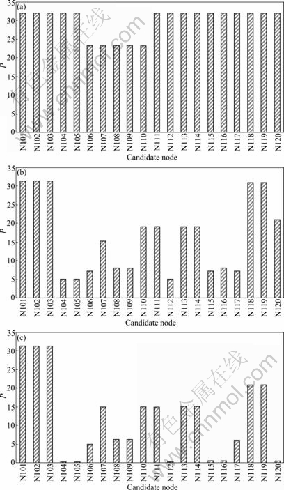
Fig. 6 Comparison of different threshold values with same injection duration: (a) 0.01 mg/L; (b) 1 mg/L; (c) 5 mg/L
3.2 Results for Scenario 2
In Scenario 2, for each possible source, independent and deterministic simulations are performed for constant injection of a contaminant with durations of 6, 12 and 24 h. In this scenario, only the circumstances under the same threshold value are considered. The same five complaint nodes are selected for identifying the source, as shown in Fig. 5. And the results are shown in Fig. 7.
Figure 7 presents the results for injection duration of 6, 12 and 24 h. The results show that injection duration has no significant effect on identification of the real pollution source with the decline of duration time. On contrary, the disparities of P value among them seem to be more and more remarkable. And it is obvious that different injection durations would yield different values for most injection nodes, however, it has no particular impact on identifying the contamination source.

Fig. 7 Comparison of different injection time with same threshold value: (a) 24 h; (b) 12 h; (c) 6 h
3.3 Results for Scenario 3
In reality, the baseline of Scenario 3 is to consider the computational cost, for the combinations of time are 2k, where k is the number of complaint nodes. The more the complaint nodes are taken into account, the more adequate the evidences for identification can be obtained. Consequently, when more complaint nodes are used to calculate the total probability, the results of identification would be more accurate and creditable. In this scenario, three cases are performed in order to estimate the effect of the number of complaint nodes on the accuracy of source identification. In the first case, five nodes are selected, just as shown in Fig. 5. In the second case, six nodes are selected, as shown in Fig. 8. And in the third case, seven nodes are elected, as shown in Fig. 9. Given that the threshold value is 5 mg/L, the results are shown in Fig. 10.

Fig. 8 Layout of selected complaint nodes for case 2

Fig. 9 Layout of selected complaint nodes for case 3
Obviously, the results shown in Fig. 10 have demonstrated the importance of the number of consumer nodes for the accuracy of source identification. In the first case, the P values among the nodes 101,102 and 103 are almost the same. It is hard to identify the real source. In the second case, the gaps among them grow up. In the last case, the differences are very significant. Consequently, given that the condition permits, it would be easy to characterize the contamination source if more complaint nodes are taken into account. However, this means that more time is needed to obtain the result.
3.4 Results for Scenario 4
In this scenario, two groups of prior probability are compared. The first group is the one used in this work. The second is based on the probability that people ingest drinking water across the daytime. It is assumed that the probability of consumer complaints is closely relevant to number of people who ingest drinking water during the contamination occurrence. The more the people ingest drinking water during contamination, the more possible the consumers complain to water utilities. Based on this assumption, the probability of consumer complaints could be reasonably estimated. The estimated probability pij at every hour is listed in Table 3. Because our purpose is to reflect the relative differences of the probability pi of each hour, the objective that these probabilities are set to various values is just to show that it is more possible for people to ingest drinking water during three meals than in other hours. Consequently, the prior probability P(Bj) is the product of each pij:
![]() (4)
(4)
where k is the total numbers of consumer complaint nodes; pij represents the prior probability of the i-th consumer complaint nodes with the j-th time combination.
A comparison of the total probability P(A) in different groups is shown in Fig. 11. It is illustrated that when the prior probability P(Bj) for each combination of time is not equal, the difference among some candidate nodes seems to decrease to a degree, for example, the total probabilities of nodes 118 and 119 are close to the ones of the first three nodes (101, 102, 103). But the difference remains significant. Nodes 101, 102 and 103 are still the most possible contamination sources from a view of magnitude of total probability. In a sense, the second group seems to be more reasonable and rigorous than the first group, for the prior probability P(Bj) is more or less associated with the number of people ingesting tap water. However, it is easy to tell the contamination source from many potential source locations, even though the model for estimating the prior probability P(Bj) has changed. In fact, the probability of each combination of time P(A|Bj) at the true intrusion location is higher than that of the ones at other locations, and complaint time mainly concentrates on the period of three meals or occurs during the day, as given in Table 2, so that with the prior probability P(Bj) changing, the total probability at the true intrusion location is still much higher than that at other locations, although the difference between them becomes smaller. Consequently, considering lack of adequate data and other uncertainties, it can still be regarded as a good way to assume that all the prior probabilities P(Bj) are equal.

Fig. 10 Comparison of different sets of nodes: (a) 5 nodes; (b) 6 nodes; (c) 7 nodes
4 Discussion
This work suggests that the proposed methodology has the ability to identify the contamination source based on consumer complaints. The results even show that a unique solution, the real contamination source, can be obtained. However, since information obtained from customer complaints is very limited and consists of a great many of uncertainties, the unique solution derived through the proposed methodology may not be the real contamination source. In the above case study, nodes 101, 102, 103 are considered as the most possible contamination sources, not just single node 101. Due to lack of adequate data, no evidence could be provided that the node with the maximum probability evaluated is not the real contamination source. However, it is possible that this case would exist. Although the examined case demonstrates the effectiveness and feasibility of the proposed method, there are additional challenges required further to research that the information employed in this work is just the location where contamination occurs and the obscure time when contamination is possible to occur. For example, within a given range of threshold values, the possible source can be further refined through increasing threshold value. At present, it is difficult to determine an effective range of threshold values to make sure that the real pollution source is not eliminated. However, there may exist some given range of threshold values within which we don��t worry about the exclusion of the true contamination source. The best solution is as follows: staring from a small enough threshold value, and then increasing the threshold value step by step until the number of the remaining possible source is acceptable. At last, the research about how to better lower the information uncertainty obtained from consumer complaints will be likely to complement the work presented here.
Table 3 Probabilities of consumer complaints in each hour


Fig. 11 Results for different prior probabilities: (a) First mode; (b) Second mode
5 Conclusions
1) Four scenarios are performed to explore the effects of threshold value, injection duration on pollution source, location of consumer complaints and different prior probabilities. Within a given range, threshold value has no influence on source identification. However, the results would be better through increasing threshold appropriately. Meanwhile, within a given range, injection duration also have no significant effect on source identification. And the source identification is not affected by the prior probability with which consumer would complaint to water utilities.
2) The number of complaint nodes which are selected for calculation would have a significant effect on the accuracy of source identification. The more the complaint nodes are involved in calculation, the more accurate the results are. This means that the number of possible pollution nodes would be narrowed further through increasing the number of complaint nodes for calculation.
3) The proposed methodology has the ability to identify the contamination source based on consumer complaints. The results even show that a unique solution, the real contamination source, can be obtained. However, since the information obtained from customer complaints is very limited and consists of a great number of uncertainties, the unique solution derived through the proposed methodology may not be the real contamination source. Note that the uncertainties of information obtained from consumer complaints are too high usually, and it is possible to exclude the true intrusion location if it aims to capture a single node blindly. Therefore, the objective of the methodology is to narrow the range of possible source, not to capture a single node or a unique solution.
4) However, to further improve the methodology and make the methodology more practicable, a number of issues which are presented in above discussions are required to be investigated in further researches.
References
[1] CRISTIANA D C, LEOPARDI A. Pollution source identification of accidental contamination in water distribution networks [J]. Journal of Water Resources Planning and Management, 2008, 134(4): 197- 202.
[2] HUANG J J, MCBEAN E A. Data mining to identify contaminant event locations in water distribution systems [J]. Journal of Water Resources Planning and Management, 2009, 135(6): 466-474.
[3] SHANG Feng, UBER J G, POLYCARPOU M M. Particle backtracking algorithm for water distribution system analysis [J]. Journal of Environmental Engineering, 2002, 128(5): 441-450.
[4] LAIRD C D, BIEGLER L T. A mixed index approach for obtaining unique solutions in source inversion of drinking water networks [C]// The World Water & Environmental Resources Congress, EWRI, Anchorage, Alaska, 2006: 16-25.
[5] PREIS A, OSTFELD A. Contamination source identification in water systems: A hybrid model trees-linear programming scheme [J]. Journal of Water Resources Planning and Management, 2006, 132(4): 263-273.
[6] LIU L, RANJITHAN S R, MAHINTHAKUMAR G. Contamination source identification in water distribution systems using an adaptive dynamic optimization procedure [J]. Journal of Water Resources Planning and Management, 2011, 137(2): 183-192.
[7] GUAN Jia-bao, ARAL M M, MASLIA M L, GRAYMAN W M. Identification of contamination sources in water distribution system using simulation-optimization method: Case study [J]. Journal of Water Resources Planning and Management, 2006, 132(4): 252-262.
[8] KUMAR J, BRILL E D, MAHINTHAKUMAR G, RANJITHAN R J. Identification of reactive contamination sources in a water distribution system under the conditions of data uncertainties [C]// World Environmental and Water Resources Congress, Tucson, Arizona, 2010: 135- 145.
[9] DAWSEY W J, MINSKER B S, VANBLARICUM V L. Bayesian belief networks to integrate monitoring evidence of water distribution system contamination [J]. Journal of Water Resources Planning and Management, 2006, 132(4): 234-241.
[10] PETER J F. Expert knowledge and its role in learning Bayesian networks in medicine: An appraisal [M]. Nijmegen: AIME, 2001: 156-166.
[11] NILSSON J J, BUCHBERGER M G, CLARK N C. Simulating exposures to deliberate intrusions into water distribution systems [J]. Journal of Water Resources Planning and Management, 2005, 131(3): 228-236.
[12] ALLMANN T P, CARLSON, ALICS K L. Modeling intentional distribution system contamination and detection [J]. J Am Water Works Assoc, 2005, 97(1): 58-61.
[13] ROSSMAN L A. EPANET 2.0 users manual [M]. Cincinnati: National Risk Management Research Laboratory, 2000: 40-41.
[14] SANCTIS A E D, SHANG Feng, UBER J G. Real-time identification of possible contamination sources using network backtracking methods [J]. Journal of Water Resources Planning and Management, 2009, 132(5): 301-311.
[15] EPANET 2.0. Toolkits. (2000). [EB/OL]. [2011-02-11]. www.epa. gov/ORD/NRMRL/wswrd/epanet.html.
[16] DAVIS M J, ROBERT J. Importance of exposure model in estimating impacts when a water distribution system is contaminated [J]. Journal of Water Resources Planning and Management, 2008, 134(5): 449-455.
(Edited by HE Yun-bin)
Foundation item: Project(50908165) supported by the National Natural Science Foundation of China
Received date: 2011-10-21; Accepted date: 2012-02-01
Corresponding author: XIN Kun-lun, Associate Professor, PhD; Tel: +86-21-65985869; E-mail: xkl@tongji.edu.cn
Abstract: A new methodology was proposed for contamination source identification using information provided by consumer complaints from a probabilistic view. Due to the high uncertainties of information derived from users, the objective of the proposed methodology doesn��t aim to capture a unique solution, but to minimize the number of possible contamination sources. In the proposed methodology, all the possible pollution nodes are identified through the CSA methodology firstly. And then based on the principle of total probability formula, the probability of each possible contamination node is obtained through a series of calculation. According to magnitude of the probability, the number of possible pollution nodes is minimized. The effectiveness and feasibility of the methodology is demonstrated through an application to a real case of ZJ City. Four scenarios were designed to investigate the influence of different uncertainties on the results in this case. The results show that pollutant concentration, injection duration, the number of consumer complaints nodes used for calculation and the prior probability with which consumers would complaint have no particular effect on the identification of contamination source. Three nodes were selected as the most possible pollution sources in water pipe network of ZJ City which includes more than 3 000 nodes. The results show the potential of the proposed method to identify contamination source through consumer complaints.
