
Trans. Nonferrous Met. Soc. China 23(2013) 1061-1071
Springback prediction for incremental sheet forming based on FEM-PSONN technology
Fei HAN1, Jian-hua MO2, Hong-wei QI1, Rui-fen LONG1, Xiao-hui CUI2, Zhong-wei LI2
1. College of Mechanical and Electrical Engineering, North China University of Technology, Beijing 100144, China;
2. State Key Laboratory of Material Processing and Die & Mould Technology, Huazhong University of Science and Technology, Wuhan 430074, China
Received 5 March 2012; accepted 15 September 2012
Abstract:
In the incremental sheet forming (ISF) process, springback is a very important factor that affects the quality of parts. Predicting and controlling springback accurately is essential for the design of the toolpath for ISF. A three-dimensional elasto-plastic finite element model (FEM) was developed to simulate the process and the simulated results were compared with those from the experiment. The springback angle was found to be in accordance with the experimental result, proving the FEM to be effective. A coupled artificial neural networks (ANN) and finite element method technique was developed to simulate and predict springback responses to changes in the processing parameters. A particle swarm optimization (PSO) algorithm was used to optimize the weights and thresholds of the neural network model. The neural network was trained using available FEM simulation data. The results showed that a more accurate prediction of springback can be acquired using the FEM-PSONN model.
Key words:
incremental sheet forming (ISF); springback prediction; finite element method (FEM); artificial neural network (ANN); particle swarm optimization (PSO) algorithm;
1 Introduction
Current market requirements for products show a need to produce a variety of parts at low cost and with a short delivery period. Incremental sheet forming, a method that can meet these needs, is in demand and has been intensively studied [1-3]. The process was conceived to provide computer numerical control (CNC) flexible sheet forming with a toolpath program to replace the need for fixed dies or tooling (Fig. 1). However, springback is a major concern in the ISF process, and an accurate prediction of springback is essential for the design of toolpaths for ISF operations [4,5].
There have been many studies about springback prediction in ISF processes. HAN et al [6] investigated springback prediction in the ISF process using a genetic neural network. However, the optimization speed was slow, and the accuracy was not very high. AMBROGIO et al [7] investigated material formability in incremental forming and, in particular, the evaluation and compensation of elastic springback through experimental investigation and explicit FEM analysis. TANAKA et al [8] investigated the negative springback phenomenon in sheet metal obtained by the incremental forward stretch forming operation, both experimentally and numerically.
However, traditional and new simulation techniques of springback prediction are laborious trial-and-error procedures, which involve long cycle times and high cost. Artificial neural network (ANN) has been proven to be a great tool for solving a wide variety of problems because of its ability to approximate non-linear functions in the absence of closed form solutions [9]. ANN provides a new way to solve complex, non-linear, polytropic springback problems. The main drawback of ANN is the need of large amounts of data for training and validating efforts. For these reasons, a FEM-ANN hybrid technique was used to generate reasonable data while avoiding expensive and time-consuming experiments.
Among the various ANNs, the back-propagation (BP) method is one of the most important and widely used algorithms. However, the conventional BP algorithm suffers from some shortcomings, such as a very slow convergence speed in training, and a tendency to get stuck in a local minima. Therefore, the present work intended to integrate ANN with particle swarm optimization (PSO) algorithm to properly determine the weights of the neural network, compensating for the defects of the BP algorithm. This method made use of the strong global and local search capabilities of the PSO and BP algorithms respectively.
In this work, the springback of the typical frustum of cone-shaped forming was investigated. Based on FEM simulation data, the prediction model of the springback was developed by the neural network and the particle swarm optimization algorithm. The predicted value of the springback in the FEM-PSONN model was in accordance with the results of the FEM.
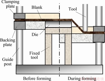
Fig. 1 Positive incremental sheet forming process
2 Experimental design and FEM analysis
2.1 Experimental setup
For the experiments described in the present work, a special 3-axis NC-controlled machine was used in the incremental sheet forming, as shown in Fig. 2. The blank was fastened by a properly designed fixture. According to the design of fixture, the thickness of the blank was 1 mm and its length and width were both 330 mm. The material of the blank was 08Al in the annealed state.
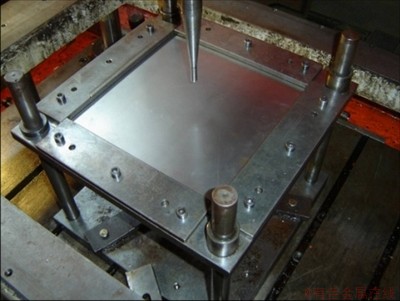
Fig. 2 Incremental sheet forming equipment
The circular die used for the experiments had a diameter of 80 mm and an edge radius of 3 mm. A spherically nosed tool (tool steel, Cr13) was used for all applied strategies. The code for the toolpath was programmed using the computer automated manufacturing module of Unigraphics NX, and the tool speed was set as 200 mm/s. Oil was applied to further minimizing friction. Figure 3 shows the parts produced by incremental sheet forming.
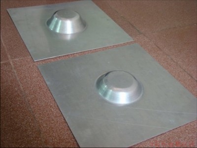
Fig. 3 Parts of incremental sheet forming
2.2 Simulation setup
A three-dimensional elasto-plastic finite element model was set up to simulate the ISF process using ABAQUS/Explicit. The results were then transferred to ABAQUS/Standard (a static implicit code) to simulate the springback step (tools removal). Because of the properties of the process, there were several nonlinearities involved in the simulation of incremental sheet forming. In addition, for the considered applications, the incremental forming process was typically in full 3D without any symmetry plane. The simulation usually required the use of a large number of elements and the tool moving along a relatively long trajectory, leading to a complicated and time-consuming finite element analysis. To validate the model, similar parameters and values of material properties were used in both the simulation and the experimental study.
2.2.1 Material and process parameters
A series of tensile tests were conducted to determine the material properties experimentally, and these material parameters were input for the simulation. The main material parameters are shown in Table 1.
ISF is a complex cold-mechanical process. There are many factors that affect the forming process, such as vertical step downs (��z) between the consecutive contours, the tool diameter (D), the sheet metal thickness (t), the wall inclination angle (��), and the final part height (H). Figure 4 shows the parameters of the ISF process.
2.2.2 Finite element model
The model used 14400 4-node shell elements (Abaqus type S4R) with five integration points through the thickness of the model. The material was assumed to be planar anisotropic following Hill��s 1948 yield criterion with kinematic hardening. The tool, partial die, clamping plate and backing plate were modelled as rigid surfaces. Coulomb��s friction law was applied, and the friction coefficients were 0.05 between the blank and the tool and 0.15 between the blank and the partial die. The contact condition was implemented through a pure Master-Slave contact algorithm. Figure 5 shows the FEM model for the process.
Table 1 Material parameters of tensile samples
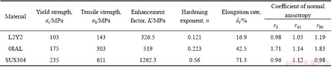
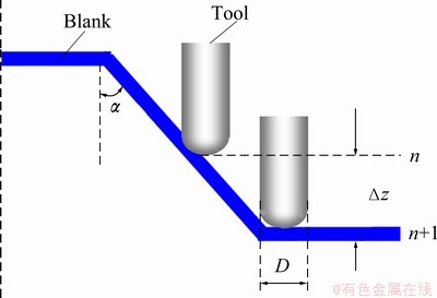
Fig. 4 Parameters of ISF process
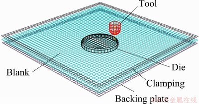
Fig. 5 FEM model for process
To synchronize the FE simulation with the experiment, the NC file from the actual experiment was imposed upon the simulation to move the forming tool. The tool movement was controlled by predefined displacement constraints in several load steps. Using an artificially high tool velocity to compensate for the real process was considered a potentially good method to shorten the simulation time. Thus the tool feed rate was artificially increased to 2000 mm/s. The simulation time was reduced significantly as the tool velocity increased by 10 fold.
2.2.3 Validation of FE model
To find out how well the simulation model of the springback was able to represent reality, a comparison with an experimental study was made. With the process parameters set as D=10 mm, ��=40��, a height of the final part of 20 mm, ��z=1 mm, and an L2Y2 aluminium sheet thickness of 2 mm, the experiment and numerical simulation of the truncated cone were performed. When the part was complete, the final shape was measured offline with a 3D laser scanner (Fig. 6) and compared with the simulation prediction (Fig. 7). As shown in Fig. 7, the experimental and numerical results were accordant.
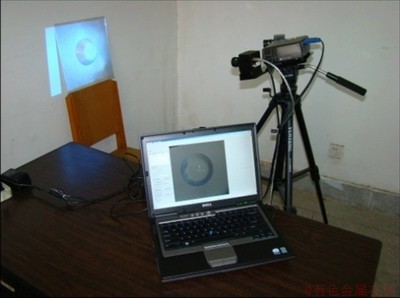
Fig. 6 Set-up for measurements using a laser scanning system
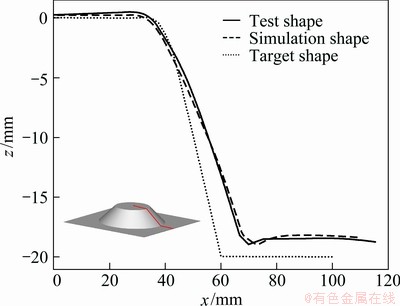
Fig. 7 Comparison of simulation and test results of a truncated cone piece symmetric cross section
The maximum deviation in the z-axis direction was 1.163 mm between test shape and simulation shape, in which that in x-axis direction was 46.421 mm. Therefore, the 3D finite element model used in this work can be considered reasonable and the results of the simulation can be considered reliable.
3 Design of process parameters based on an orthogonal experiment
Orthogonal experimental design is one of the basic means of Taguchi parameter design based on Latin Square theory and Group theory, and it can be used to design multi-factor tests. As a result, the size of the full permutation and combination of experiments concerning various factors could be greatly reduced; therefore, it is considered to be an excellent experimental design method. In this work, the parameter design of orthogonal experimentation was used to provide the sample for the neural network.
3.1 Experiment index of a workpiece springback of incremental sheet forming
To analyze the sheet springback of incremental sheet forming, as shown in Fig. 8, ���� (angle difference before and after springback in the symmetrical section of the truncated right angle cone workpiece ) was taken as the experiment index.
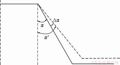
Fig. 8 Schematic diagram of springback angle of incremental sheet forming
In this work, the resilience value was assessed by the springback angle, as shown in Fig. 8. In the figure, the solid line is the target-shape contour of the incremental sheet forming, the dotted line is the actual-shape contour after springback, �� is the sidewall angle before springback, ���� is the sidewall angle after springback, and ���� is the difference between �� and ����, which ultimately represents the springback angle of the workpiece.
3.2 Orthogonal experimental design
According to the characteristics of incremental sheet forming and our attempts to emulate practical production conditions as closely as possible, six main factors affecting the experiment index were chosen as experimental design variables (the ratio of yield strength to the elastic modulus of the sheet, the sheet thickness, the diameter of the tool head, the forming working height, the half-apex angle of forming parts, and the monolayer feeding quantity of the tool head), and interaction between design variables was ignored. The abbreviations of every factor in sequence were A, B, C, D, E, F, in the context of the possible value range for each factor; together with the professional knowledge and the FE simulation results, this approach allowed three levels of every design variable (factor) to be acquired as shown in Table 2.
The orthogonal table, L18(37), consisting of three levels of six design variables each, was used to design a set of experiments. Therefore, 18 calculation combinations with orthogonal conditions were constructed, and 18 FE simulations of incremental sheet forming were generated.
3.3 Orthogonal experiment simulation results and analysis
The corresponding experimental factors were combined with ABAQUS to create 18 simulations of incremental sheet forming, with the orthogonal experiment results shown in Table 3.
3.3.1 Range analysis
The range analysis method was used to calculate the range value (R) of each column in the orthogonal table using mathematical statistical method. The range was used to determine the primary and secondary order of influence factors. Factors with large range values were significant, while those with small range values were not. The range values were calculated from Table 4. The order of the ranges was R5>R4>R3>R1>R6>R2. Therefore, the order of impact of each factor on the experiment index was, from the largest to the smallest, E, D, C, A, F, and B.
Table 2 Levels of analyzing factors in a digital incremental sheet forming springback
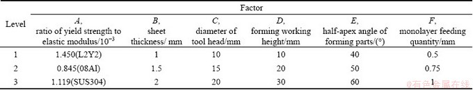
Table 3 Orthogonal experiment results
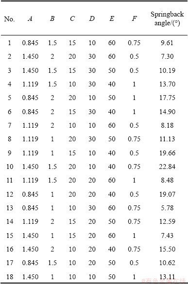
Table 4 Range analysis of process parameters on springback
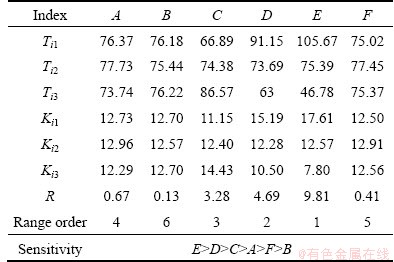
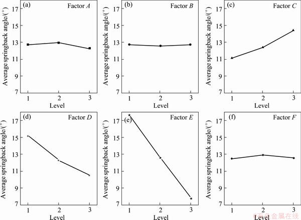
Fig. 9 Impact of each factor and level on springback
The average simulated values of the springback angle of each factor at different levels are shown in Fig. 9. The half-apex angle of forming parts was the angle most sensitive to springback. When the load was partially uninstalled, there was an increase in the half-apex angle of the forming parts, thus the force released by the elastic deformation ascended, and the springback became more obvious. The forming working height was also very sensitive to the springback. Because of the partial increase of the plastic deformation of the sheet, springback decreased. The diameter of the tool head was also sensitive to the springback. The larger the diameter of the tool head, the more the residual stress was released when uninstalling the load, thus the springback increased. As shown in Fig. 9, the curve of factor C increased monotonically. The material parameters determined the properties of the material itself. Though the sensitivity was not obvious, it still had a decisive impact on the results. However, the monolayer feeding quantity of the tool head and the sheet thickness were not very sensitive to springback.
3.3.2 Variance analysis
Although the range analysis was intuitive and easy to calculate, the accuracy of the calculations was insufficient. To overcome the low accuracy of the range analysis, the experimental data were processed by variance analysis.
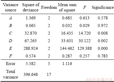
It can be observed from Table 5 that the variance caused by the change of the half-apex angle of the forming parts accounted for 72.84% (288.924/396.648) of the variance. The change of the forming working height accounted for 16.96% (67.263/396.648), the change of the diameter of the tool head accounted for 8.29% (32.870/396.648), the change of the material factors accounted for 0.35% (1.369/396.648), the change of the monolayer feeding quantity of the tool head accounted for 0.14% (0.574/396.648), and the change of the sheet thickness only accounted for 0.016% (0.065/396.648). Therefore, the order of impact of each factor on the experiment index was E, D, C, A, F, and B. Thus, the significance analysis conclusions for each factor using variance analysis were in accordance with the conclusions by the range analysis.
Table 5 Variance analysis
4 Model of springback prediction based on neural network of a particle swarm
In the incremental sheet forming process, the springback prediction has a great influence on the accuracy of the forming parts�� final shapes. As a result, fast and accurate springback prediction is particularly important. For most metal plastic forming processes, a complete and accurate analytical model for calculating springback quantity was unable to be established because numerical simulations or empirical formulas were used to meet the needs of the engineering technology. However, this method is limited regarding calculation accuracy and speed. Therefore, it is very important to find a reasonable and scientific method to calculate the springback accurately in incremental sheet forming processes.
The error back propagation neural network algorithm has a simple structure, is self-learning, and uses parallel processing [10]. The BP algorithm has the advantage of optimization with precision, but it also has some shortcomings, such as the tendency to fall into local minima, a slow convergence rate and a chance to cause vibration effects. Therefore, in this section, the strategy of combining artificial neural networks and the particle swarm optimization algorithm was used, and a prediction model of springback quantity of the incremental sheet forming using the combined PSONN (particle swarm optimization and neural networks algorithm) was established. The model effectively solved the local convergence of a traditional BP network and improved the learning speed and prediction accuracy.
4.1 BP and its improved model of neural networks
The BP neural network can adopt the error back-propagation learning algorithm and use the gradient searching technique to achieve the minimization of the mean square error of the actual output and the expected output.
The BP learning process is as follows: the input value of the network from the input layer passes to the hidden layer through a weighting treatment, and then the output of the hidden layer is obtained from the operation of the activation function of the hidden layer. The output value of the weighted hidden layer is transmitted to the output layer after the weighting treatment, and then the output value of the network is obtained after the operation of the activation function of the output layer. The error is back propagated, and the network connection weights between layers and the neuron threshold are modified, layer by layer, to decrease the error. Training is repeated until the errors meet the accuracy requirements [11-13].
However, the BP algorithm has the disadvantages of easily falling into the local minimum and a slow convergence speed. To counter these disadvantages, an additional momentum method and an adaptive learning rate were used.
4.2 Hybrid algorithm model of particle swarm and neural network
The particle swarm optimization (PSO) algorithm is a global optimization algorithm based on group evolution, and it can obtain a near optimal global solution, without falling into a local minima. In addition, its optimization process does not rely on gradient information and its high search efficiency is robust [14-16].
To overcome the shortcomings of the BP algorithm, which easily falls into a local minima and has a slow convergence rate, and to improve the convergence speed and accuracy of the springback-prediction model, this section applies the particle swarm optimization algorithm to train and model the artificial neural network with the goal of constructing a model with a faster convergence speed and a higher prediction accuracy, obtaining a better compensation effect.
4.2.1 Particle swarm algorithm
In the PSO algorithm, each solution to the optimization problem is used to search for a ��bird�� in space that we call a particle. Each particle has its own position and velocity (which determines the direction of flight and distance), and proper values for these parameters are determined by the optimization function. Finally, the particle swarm follows the optimal particles to search in the solution space.
4.2.2 Hybrid algorithm for particle swarm neural networks
The network learning algorithm work flow is as follows:
Step 1: To determine the algorithm parameters, firstly the size of the PSO particle number m must be determined. Secondly, we must set the initial inertia weight w, the connection thresholds of neural network ��ik and ��kl, the maximum allowable number of iterations kmax, and the random variables c1 and c2, as well as initializing iterations k=1.
Step 2: The term {wik} is used to express the connection weights between the input layer and the hidden layer. {wkl} expresses the connection weights between the hidden layer and the output layer. The weights of the neural networks and the connection variables are coded as follows: x={wik, wkl, ��ik, ��kl}.
Step 3: Initialization. In a given interval, when initializing randomly connection weights, the connection variable is usually initialized to a random [0,1] interval of real numbers. Therefore, the PSO is initialized to generate PSO{xi(0), i=1, 2, ��, m} on behalf of m types of different weights of the neural network, and is used as the initial solution set of the PSO algorithm. The PSO algorithm training weight speed is initialized randomly.
Step 4: The particle xi, which corresponds to a neural network output value and the expected mean variance minimum, is targeted using Eq. (1) to derive the fitness value f(Xi) of individual xi, and to initialize Gbest and Pbest.
 (1)
(1)
 (2)
(2)
where f(X) expresses the fitness of X; E(X) expresses the error level after the training of the BP network results expressed by individual X, here decided by Eq. (2); dj(k) is the desired output and selected as the objective function of the weight update; m is the number of output layer nodes.
Step 5: The current fitness  of each particle in PSO is compared with the individual extreme value
  . If the current fitness of a particle is better than the individual extreme value before the iteration, then the individual extreme value
  , where k represents the number of iterations, must be updated. Otherwise,
  .
.
Step 6: Update the global extreme value.  ,
,  of all the individual points, and the optimal fitness of the individual extreme values shall be used as the global extreme values.
Step 7: Optimization of the particle position. The formulas (3) and (4) are used to update the velocity vi and position xi of each particle.
 (3)
(3)
 (4)
(4)
where n is the dimension of solution space, namely, the number of independent variables; d is the n-dimension in the d-dimension; k is the current evolution algebra;  and
and  are limited factors of displacement changes, often referred to as the acceleration weighting coefficient; ��(k) is the inertia weight. r1 and r2 are random numbers which change in the scope of [0,1]. At the same time, in the evolutionary process, in order to prevent the particles from flying out of the search space, usually the Vi will be limited to a certain extent, that is
  .
.
Step 8: The fitness evaluation of new particle populations is generated by iterations. To determine whether the algorithm arrives at the maximum number kmax of iterations, or whether the training error E is less than the specified minimum error requirement, the iteration and output of the optimal solution of neural network are stopped. Otherwise, k=k+1, and it can be returned to step 4.
Step 9: To calculate the neural network output using pg (obtaining the global optimum value eventually), the network weights and thresholds optimized for the particle swarm as the network initial weights and thresholds of the BP algorithm are taken, in accordance with the BP algorithm for training learning, which is to be used for the PSO-ANN springback prediction models.
5 Simulation experiments and results analyses
To examine the effects of network learning using the improved PSO algorithm on the simulation experiments, we took the orthogonal experimental design data as sample sets using the standard BP network, the improved BP and PSO-BP to learn and test the samples, to evaluate their results, and to check the validity of the improved algorithm.
5.1 Parameter settings of neural network model
The neural network structure of springback prediction in incremental sheet forming is shown in Fig. 10.
As observed in Fig. 10, there are 6 inputs and 1 output in the network, and the choice of the number of hidden layer neurons is a very complex issue, according to the empirical formula  , where a is the number of the output neurons, b is the number of the input neurons, and c is a constant between 1 and 10. This finding highlighted the complexity involved in setting up the 11 nodes in the hidden layer when investigating the corresponding prediction time and accuracy. Eventually, the intelligent optimization model was identified to have a network structure of 6-11-1.
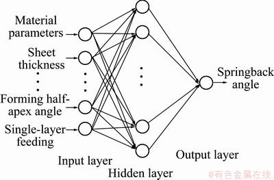
Fig. 10 Topology structure of incremental forming springback prediction neural network
In this work, the BP algorithm, the improved BP algorithm and the neural network model for springback prediction based on particle swarm optimization (PSO-ANN) were developed in a MATLAB language environment. For the standard BP algorithm training, the initial and threshold values were set randomly between [-1, 1] and the learning rate was set to be ��=0.57. The improved algorithm used an initial learning rate of ��=057 and a momentum factor of ��=0.85. In the process of learning, formulas (5) and (6) were used to adjust the learning rate and momentum factor.
 (5)
(5)
 (6)
(6)
where is the amendment of the weight and threshold for the (k-1) time; �� is the momentum factor.
When the simulation of the prediction model of the springback samples with the PSO-ANN algorithm was performed, the initial population size was set to be m=100, the network structure was set to be 6-11-1, and the simulation used a total of 77 weights and 12 thresholds; therefore, the search space for each particle in the particle swarm algorithm was 89-dimensional. Additionally, the initial inertia weight �� was 0.8, with a linear decrease in the number of iterations to 0.4, a learning factor of c1=c2=2, a maximum speed vmax=0.5, a maximum number of iterations Gmax=400, and a default error of 0.004. The algorithm was repeated several times, selecting different iterations and population sizes, choosing the particles of the highest fitness as the neural network initial rights (threshold) values, and then using the standard BP algorithm with a learning rate of ��=0.57 for a training target error of 0.002.
5. 2 Analysis of simulation results
To test the BP algorithm in the CNC incremental sheet forming springback prediction system, we used the standard BP algorithm, the improved BP algorithm and the PSO-ANN algorithm for training models for the performance of the convergence speed, the precision of the model predictions, and the incremental forming springback prediction, respectively, of the artificial neural network.
5.2.1 Comparison of network convergence performance
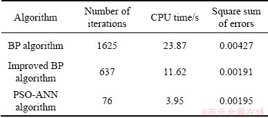
A comparison of the convergence performance using the BP algorithm, the improved BP algorithm and the PSO-ANN algorithm is shown in Table 6.
Table 6 Performance comparison of three algorithms
The error convergence curve shown in Fig. 11 is the convergence of the training network adopted by the BP algorithm, the improved BP algorithm and the PSO-ANN algorithm.
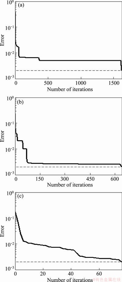
Fig. 11 Error convergence curves of BP algorithm (a), improved BP algorithm (b) and PSO-ANN algorithm (c)
As observed from Fig. 11, at 1625 iterations, the BP algorithm started to step into a local minimum with an error accuracy of 0.004127, and the convergence did not meet the requirements of the error precision. The number of iterations of the improved BP algorithm was 637. The running time of the PSO-ANN algorithm was 3.95 s, and the number of iterations was 76. In the case of the algorithms having the same accuracy, the PSO-ANN algorithm converged fast out of the three types of network training algorithms.
5.2.2 Comparison of network prediction results
To analyze the resilience of the volume prediction data of the training samples, the prediction results of the PSO-ANN hybrid algorithm, the BP algorithm and the improved BP algorithm were compared, as shown in Table 7.
As observed in Fig. 12 and Table 7, the artificial neural network model based on the standard BP algorithm, the improved BP algorithm and the PSO-ANN algorithm for springback prediction in incremental forming has achieved good results. Concerning the precision of the predictions, the maximum relative error of the BP network model was 6.868%, the average absolute error was 3.106%, and the mean root square error was 1.159%. In the improved BP network model, the average absolute prediction error was reduced to 2.257%, and the mean root square error was 0.8 %. The minimum relative error of the PSO-ANN model was only 0.017%, the maximum relative error was 3.069%, the average absolute error was reduced to 1.118%, and the mean root square error was 0.443%.
Table 7 Comparison of prediction results of neural network algorithms
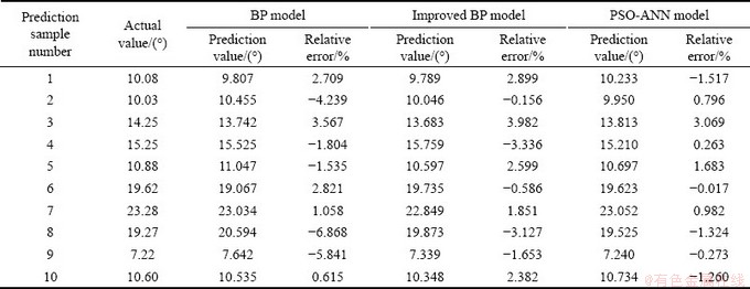
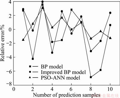
Fig. 12 Neural network prediction error curve
It was observed that the use of the BP algorithm of the neural network had a good predictive ability, and its degree of fitness was better. However, due to the inherent defects in the BP network (the slow convergence and tendency to fall into local minimum points), its predictive power was inferior to the PSO-ANN algorithm. This was because the particle swarm algorithm had the feature of global search, which was used to optimize the BP network weights, and the threshold value of the BP algorithm to overcome the inherent defects, while highlighting the local optimization ability of the BP algorithm, thus achieving a fast convergence rate and increased accuracy. Simulation results showed that among the three algorithms, the testing error of the model for the PSO-ANN algorithm was the smallest and the network generalization ability was the best. It had the highest prediction accuracy and was better than the other two algorithms in the optimal approximation of the non-linear relationship between the incremental sheet forming springback and the influence factors.
6 Conclusions
1) The three-dimensional elastoplastic finite element model of incremental sheet forming processes was generated. The contrast and analysis of the simulation and test results of the example showed that the finite element model was correct and reasonable; further, the springback angle was found to be in accordance with the experimental results.
2) An incremental sheet forming springback prediction model based on the particle swarm optimization neural network was established, the particle swarm optimization (PSO) algorithm was used to optimize the weights and thresholds of the neural network model, and the neural network was shown to have the ability to be trained based on available FEM simulation data.
3) The samples of the neural network prediction model for springback prediction were tested using the standard BP algorithm, the improved BP algorithm and the PSO algorithm. Through a comparative analysis with the prediction results, it was observed that the back propagation neural network prediction model of the PSO algorithm proposed improved not only the prediction accuracy, but also the learning speed of the network.
References
[1] MATSUBARA S. Incremental backward bulge forming of a sheet metal with a hemispherical head tool [J]. Journal of the Japan Society for Technology of Plasticity, 1994, 35: 1311-1316.
[2] AMINO H, RO G. 3 Dimensions digital control technology: Present situation of dieless NC forming [J]. Journal of the Japan Society for Technology of Plasticity, 2004, 45(526): 868-872.
[3] MO Jian-hua, HAN Fei. State of the arts and latest research on incremental sheet NC forming technology [J]. China Mechanical Engineering, 2008, 19(4): 491-497. (in Chinese)
[4] JESWIET J, MICARI F, HIRT G, BRAMLEY A, DUFLOU J, ALLWOOD J. Asymmetric single point incremental forming of sheet metal [J]. CIRP Annals��Manufacturing Technology, 2005, 54(2): 88-114.
[5] AMBROGIO G, FILICE L. A simple strategy for improving geometry precision in single point incremental forming [C]// Proceedings of the 8th International Conference on Technology of Plasticity (ICTP 2005). Verona, Italy, 2005: 357-358.
[6] HAN Fei, MO Jian-hua, GONG Pan. Incremental sheet NC forming springback prediction using genetic neural network [J]. Journal of Huazhong University of Science and Technology: Nature Science Edition, 2008, 36(1): 121-124. (in Chinese)
[7] AMBROGIO G, COSTANTINO I, de NAPOLI L, FILICE L, MUZZUPAPPA M. Influence of some relevant process parameters on the dimensional accuracy in incremental forming: A numerical and experimental investigation [J]. Journal of Materials Processing Technology, 2004, 153-154: 501-507.
[8] TANAKA S, NAKAMURA T, HAYAKAWA K, NAKAMURA H, MOTOMURA K. Experimental and numerical investigation on negative springback in incremental sheet metal forming [C]//12th International Conference on Metal Forming. Cracow: Verlag Stahleisen MBH, 2008: 55-62.
[9] SWADESH S K, KUMAR D R. Application of neural network to predict thickness strains and finite element simulation of hydro-mechanical deep drawing [J]. The International Journal of Advanced Manufacturing Technology, 2005, 25: 101-107.
[10] RUMELHART D E, WILLIAMS R J. Learning representations of back-propagation errors [J]. Nature, 1986, 323: 533-536.
[11] WU Wei, WANG Jian, CHENG Ming-song, LI Zheng-xue. Convergence analysis of online gradient method for BP neural networks [J]. Neural Networks, 2011, 24(1): 91-98.
[12] ZHOU Shao-qian, DING Li-xin, ZHANG Jian, TANG Xin-hua. Linearization learning method of BP neural networks [J]. Wuhan University Journal of Natural Sciences, 1997, 2(1): 35-39.
[13] YANG Bin, LIU Li-hua, ZHANG Shao-kun. Fitting theory and method of hyper-elastic materials�� nonlinear constitutive relations base on BP neural network [J]. Applied Mechanics and Materials, 2012, 137: 36-41.
[14] KENNEDY J, EBERHART R C. Particle swarm optimization [C]// Proc IEEE International Conf on Neural Networks. Perth: IEEE Piscataway, 1995: 1942-1948.
[15] JIA Dong-li, ZHENG Guo-xin, QU Bo-yang, KHAN M K. A hybrid particle swarm optimization algorithm for high-dimensional problems [J]. Computers & Industrial Engineering, 2011, 61(4): 1117-1122.
[16] SUN Guang-yong, LI Guang-yao, CHEN Tao, ZHANG Yong. Application of multi-objective particle swarm optimization in sheet metal forming [J]. Journal of Mechanical Engineering, 2009, 45(5): 153-159. (in Chinese).
����FEM-PSONN�����İ�Ľ������λص�Ԥ��
�� ��1��Ī����2�����ΰ1�����1��������2������ΰ2
1. ������ҵ��ѧ ���繤��ѧԺ������ 100144��
2. ���пƼ���ѧ ���ϳ�����ģ���������ص�ʵ���ң��人 430074
ժ Ҫ���ڰ�Ľ������ι����У��ص���Ӱ���Ľ������μ�������һ����Ҫ���ء�Ϊ����ư�Ľ������ι����еĹ���·������ȷ��Ԥ��Ϳ��ƻص����б�Ҫ��������ά����������Ԫģ��ģ�⽥�����ι��գ������ص��ǵ�ģ������ʵ�������бȽϣ�����Ǻϵúܺã�˵��������Ԫģ������Ч�ġ����һ������˹������������Ԫ���ļ���(FEM-PSONN)ģ�ⲢԤ�ⲻͬ���ղ������Ƽ��Ļص�������������Ⱥ�Ż��㷨�Ż�������ģ�͵�Ȩ�غ���ֵ���������������Ԫģ���������������ѵ���������������FEM-PSONNģ���ܸ�ȷ��Ԥ��ص����ؼ��ʣ���Ľ�������(ISF)���ص�Ԥ�⣻����Ԫ��(FEM)���˹�������(ANN)������Ⱥ�Ż�(PSO)�㷨
(Edited by Hua YANG)
Foundation item: Project (50175034) supported by the National Natural Science Foundation of China
Corresponding author: Fei HAN; Tel: +86-10-88803702; E-mail: hanfei@ncut.edu.cn
DOI: 10.1016/S1003-6326(13)62567-4
Abstract: In the incremental sheet forming (ISF) process, springback is a very important factor that affects the quality of parts. Predicting and controlling springback accurately is essential for the design of the toolpath for ISF. A three-dimensional elasto-plastic finite element model (FEM) was developed to simulate the process and the simulated results were compared with those from the experiment. The springback angle was found to be in accordance with the experimental result, proving the FEM to be effective. A coupled artificial neural networks (ANN) and finite element method technique was developed to simulate and predict springback responses to changes in the processing parameters. A particle swarm optimization (PSO) algorithm was used to optimize the weights and thresholds of the neural network model. The neural network was trained using available FEM simulation data. The results showed that a more accurate prediction of springback can be acquired using the FEM-PSONN model.
